Hi again! The question I’m about to pose is one that, I’m reliably informed, clears rooms at cocktail parties.¹ But I think it sits at the foundation of why institutions are so hard to reform — and why the people who try to reform them so often end up making things worse. That’s for next time, though. Today, I want to talk about games.

Taking Your Ball and Going Home

Here’s a scene everyone recognizes. Two kids are playing a game — basketball, say. One of them is losing. So he picks up the ball, says “this is stupid,” and goes home (note: he never says, “I forfeit the game,” maybe he was in a hurry?) Anyway, pragmatically at least, “uhh, game over.” Sounds like a lot of (mostly less fun) games I have played in life. (I won’t tell you which character I was playing, but I will admit/confess that I have played both “roles,” so to speak. I’m a “double threat,” I suppose. Is that a compliment to myself?)

Now: what just happened, strategically? Within the rules of basketball, there is no explicit provision for this exact situation. Instead, the “rules of basketball” understandably tell you “what happens” when you shoot (depending on whether it “goes through the hoop,” for example), when you foul, when the clock runs out. They do not tell you what happens when a player picks up the ball and leaves the court, never to return. This action is, formally speaking, outside the game. Your first instinct might be: “Well, obviously — he loses. He quit.” And that’s a perfectly reasonable/”practically accurate” interpretation. But notice that “he quit, and therefore he loses” is your (and, yes, most of society’s) inference, not the rules’ literal interpretation.

To make this less ethereal, suppose instead the kid says, “I’m so sorry — my parents are here, I have to leave!” Should that kid lose because of his parents’ timing/schedules? (And, in spite of my inclinations, no, “don’t be a stickler right now.” Yes, that’s about to get “ironic AF”.)

The rules of basketball define how you score and how the clock works; they don’t contain a general provision for “a player decided to leave and never come back.” You’re filling the gap with common sense — and common sense, as we’ll see, is doing a lot of heavy lifting that the formal rules cannot. Let me push on this with a darker example, because I think it reveals something important.

The Penalty Ceiling

Suppose, in the course of an NBA game, you want to prevent an opponent from scoring. You could commit a blocking foul. You could commit a hard foul — a flagrant foul, in the NBA’s terminology.² The NBA distinguishes two levels: a Flagrant 1 (“unnecessary contact”) gets you two free throws and possession for the other team, while a Flagrant 2 (“unnecessary and excessive contact”) adds an ejection. That’s where the ladder ends. There is no Flagrant 3. So: what if, instead of committing a hard foul, you grab the opposing player and strangle him? Within the formal rules of basketball, the in-game consequence is… [flips through pages speedily….] well, it’s identical to a Flagrant 2 foul. Ejection. Two free throws. Possession. The rules literally cannot distinguish, in terms of game outcomes, between a very hard basketball play and attempted murder. Everything above the Flagrant 2 ceiling looks the same to the game. Criminal law handles the strangulation, of course — but that’s an external enforcement system, a different “game” entirely. Within the four corners of basketball’s rules, the marginal in-game cost of escalating from a hard flagrant to actual assault is zero.³

Now, you might (yes, quite reasonably) think: “Fine, but no one actually strangles an opponent during a basketball game. The criminal law deters that.” True. But the fact that you need to invoke an entirely separate system of rules (here: “the rules of the legal system”) to handle actions that are physically possible within the game is essentially precisely the point. From a logical perspective, the rules of the “game of basketball” themselves have a ceiling,⁴ and above that ceiling, deterrence vanishes.

This matters beyond basketball. Consider: why have police unions historically resisted making the penalty for assaulting an officer as severe as the penalty for killing one? It’s not squeamishness. It’s strategy. If assaulting a cop carries ten years and killing a cop carries life, then a suspect who has already committed the assault faces an enormous marginal cost for escalating further. The gradient protects the officer. But if both carry life? The marginal cost of escalation drops to zero. A suspect who has already crossed the assault threshold faces no additional deterrence against killing. The punishment structure only deters escalation when there’s room to escalate into.

The general principle: any finite penalty schedule creates a flat region at the top where marginal deterrence fails. And raising the ceiling doesn’t solve the problem — it just moves the flat region higher. You haven’t eliminated the zone where deterrence vanishes; you’ve simply changed where (i.e., “conditional on what action?”) the deterrence “has its bite.”

And there’s a second problem with “if you do X, you lose” — one that is, if anything, even more fundamental. Everything I’ve said so far implicitly assumes a two-player game. In a (zero-sum)⁵ two-player game, “you lose” means “your opponent wins,” and since you have exactly one opponent, this is unambiguously bad for you. The fix might fail for other reasons, but at least it’s a punishment. Add a third player and even this breaks down. “You lose” no longer determines who wins — it just removes you from contention. And the question of which remaining player benefits from your removal is now a strategic variable. If you prefer Player C to Player B, and your continued participation is helping B more than C, then losing is not a punishment — it’s a gift to your preferred outcome. “If you break this rule, you lose” becomes, in effect, “if you break this rule, you get to kingmake.”⁶ The penalty has been tranformed from a deterrent into a strategic instrument, and, having assigned a definite/predictable outcome to the violation in question, the rules have no way to prevent (or, somewhat ironically, deter) this type of behavior. They did exactly what they were supposed to do. The problem is that what they were supposed to do “isn’t enough” — or more appropriately, they are not incentive compatible within the game itself.

This is not that exotic, of course. In sports, it’s called tanking: a team deliberately loses late-season games to secure a more favorable draft pick or dodge a stronger playoff opponent. In elections, it’s strategic withdrawal: a candidate drops out not because they can’t win, but to determine who among the remaining candidates does. In legislatures, it’s the entire logic of strategic voting and logrolling.

Simple and universal point: whenever “a game” has three or more players, even the declarative “you lose” outcome is no longer necessarily the worst possible outcome. How you lose, and when you lose, and who benefits from your loss are all strategic variables that the rules have handed you.⁷ The penalty, intended to close the game, has opened it. (Readers of this blog will note the family resemblance to a certain famous theorem about what happens when you have three or more alternatives: it sort of rhymes with “Mia Farrow.” We’ll come back to this.) I want to convince you that this problem is not trivial at all. In fact, I think it’s a deep problem, one that connects to some of the most important results in mathematics, and political economy.

The Chessboard, Overturned

Consider chess. Chess is, compared to basketball in the driveway, a remarkably well-specified game. The rules define every legal move, every legal position, and every terminal outcome (checkmate, stalemate, draw by repetition, and so on). Chess even has a formal provision for one action that might seem “outside” the game: resignation. If you tip over your king, the game ends and your opponent wins. Clean, elegant, formally complete. But now imagine a player who, upon finding herself in a losing position, sweeps all the pieces off the board and onto the floor. What happened? Not a resignation — she didn’t tip her king. Not a checkmate. Not a draw. The rules of chess, so carefully specified, have nothing to say about this. And here’s what’s interesting: it’s not obvious what they should say. The most natural response — the one most people jump to — is: “Well, obviously she loses. Flipping the board is just resignation with theatrics. We can infer that she wanted to concede and was simply… efficient about it.” And in a single game of chess, maybe that resolution works well enough. But notice what it’s doing: it’s interpreting a physical action (scattering pieces) as a strategic action (resignation) by reasoning about the player’s intent. The rules of chess say nothing about intent. We’re filling the gap with inference — and inference, as we’re about to see, opens its own can of worms.

The Game Within the Game

Here’s where it gets interesting (Ed: …Finally?). Suppose our chess player isn’t playing a single game. She’s playing a best-of-seven match. She’s down a game, and the current game — game 3 — is going badly. She has two options within the formal rules: play on to the bitter end, or resign. But these two options are strategically different in the context of the match, even though they produce the same outcome in game 3 (she loses). Playing to the bitter end reveals information — about her style, her preparation, her responses to specific positions — that her opponent can exploit in games 4 through 7. Resigning early conceals that information. Accordingly, the timing and manner of her concession is itself a strategic variable, one that the rules of chess (which govern individual games) don’t acknowledge at all. The match is a game; each game within the match is a game; and the two levels interact in ways that neither level’s rules fully capture. Now: is it “legitimate” for a player to play badly — or concede early — in game 3 in order to improve her chances in game 4, 5, 6, and/or 7? While I play chess, I’m not serious at it (Ed: you mean you’re not that good at it?) That said, I suspect that most chess players would say this offends the spirit of competition (to understand why, ask yourself, “does anybody think being described as tanking something is a compliment?) But the rules of a best-of-seven match, as typically specified, say nothing about it. We’re back in the gap between what the rules formally cover and what is physically (and strategically) possible.

What Poker Understands

This is a good moment to note that at least one common game does understand the problem we’re circling around — or at least one important dimension of it. In standard Texas Hold’em, when all of your opponents fold, you win the pot. You may then show your cards to the table, but you are explicitly not required to. This is a rule about information, and it is one of the rare cases where a game’s designers grasped that the strategic management of private information is itself part of the game. Whether you show a bluff, show a strong hand, or show nothing at all is a decision with consequences for future hands — and the rules protect your right to make that decision. Most rule systems are not nearly this sophisticated. They either ignore the information dimension entirely (chess doesn’t care (or, more accurately, is realistic about the fact that it “can’t measure”what you were “thinking” about doing) or — and this is the case that will matter most for us — they try to compel disclosure, and immediately discover that compelled disclosure is extraordinarily hard to enforce.

Belichick’s Injury Reports (and Other Mendacities)

Which brings us to the NFL, and to a man who made a career out of finding the gaps between what rules say and what rules mean. The NFL requires teams to publicly disclose player injuries before each game. The purpose is transparent: betting markets, opposing teams, and fans should have access to the same basic information about who’s healthy and who isn’t. The rule was designed to “level the playing field” — to prevent teams from gaining a strategic advantage by concealing private information about their own roster. This is, on its face, a reasonable rule. It is also exactly the kind of rule that is most vulnerable to manipulation, because it attempts to regulate something — private information — that the regulator cannot directly observe. The NFL can see what a team reports. It cannot easily verify whether the report is accurate. And so Bill Belichick, with characteristic precision, listed half his roster as “questionable” every single week. Technically compliant. Informationally useless. The rule required disclosure; Belichick disclosed — in a way that conveyed nothing. The spirit of the rule was defeated by the letter of the rule, and the letter couldn’t be tightened without creating new problems. (What does “accurate” mean? Must a team disclose a player’s private medical details? Who adjudicates disagreements about severity?) Notice the irony: the injury disclosure rule was created specifically to prevent teams from “gaming the game” with private information. But the rule itself became the game that got gamed. This isn’t a bug in the NFL’s rule-writing process. I think it’s a theorem — and we’re about to see it again.

Belichick’s Safety

Let me give you a second Belichick example, because one might be an anecdote but two starts to look like a pattern (and, yes, I am both a proud Tarheel and Steelers fan, so I am not “unbiased” with respect to Billy B). In a 2003 NFL game, Belichick’s New England Patriots were leading the Denver Broncos late in the game. Facing a 4th down deep in their own territory, the conventional play would be to punt. But Belichick did something that, at the time, struck many observers as bizarre: he had his punter intentionally run out of the back of the end zone, conceding a safety — two points for Denver. Why? Because a safety, unlike a punt, is followed by a free kick from the 20-yard line, which typically travels farther and is harder to return than a punt from deep in your own end zone. Belichick wasn’t breaking any rules. He was following them. But he was exploiting a feature of the rule mapping — the relationship between safeties and free kicks — that the rules’ designers almost certainly never intended as a strategic option. The rules said: “if a safety occurs, the following happens.” They assigned an outcome to the event. And that assigned outcome, in the right circumstances, made deliberately causing the event profitable. This is not a curiosity. This is a theorem.

Gibbard-Satterthwaite, in Football Pads

The Gibbard-Satterthwaite theorem, one of the foundational results in social choice theory, tells us (informally) that any sufficiently rich system of rules that isn’t dictatorial — that is, any system where more than one person’s actions matter — is manipulable. There exists some situation in which some agent can achieve a better outcome by acting contrary to the system’s intended purpose. Both of Belichick’s exploits are Gibbard-Satterthwaite in football pads. The NFL’s rules are “sufficiently rich” (they cover a complex, multi-agent strategic environment) and non-dictatorial (both teams’ actions matter). So the theorem guarantees that there exist situations where a team can benefit by doing something the rules didn’t envision as a strategic choice. The intentional safety was always there, latent in the rule book, from the moment the safety/free kick provision was written. The meaningless injury report was always available, from the moment the disclosure rule was written. It just took decades — and a coach who modeled the game differently than the rule designers — to find them. And notice the computational point: these exploits were hard to find. Not hard in the sense of requiring genius (though Belichick is a genuinely brilliant strategic mind), but hard in the sense that the space of possible rule interactions is vast, and most people never think to search it. The manipulability is guaranteed by theorem; the discovery of any particular manipulation is a search problem of potentially enormous complexity.

The Trilemma

Now let’s go back to our ball-taker and our chessboard-flipper and think about what a game designer could do about these “outside” actions. I think there are exactly three options, and none of them is satisfactory. 

Option 1: Leave the action outside the game. The rules simply don’t address it. This is the status quo for chessboard-flipping. The game is formally incomplete: there exist feasible actions with no assigned outcome. This might seem acceptable — we handle these situations with social norms, tournament rules, or just the general understanding that you’re not supposed to do that. But “not supposed to” is doing an enormous amount of work here, and it’s not part of the formal game. We’ll come back to this. 

Option 2: Assign the action a bad outcome. “If you flip the board, you lose.” This is the most natural response, and it’s what most rule systems try to do — define penalties for rule-breaking. But here’s the problem: the moment you assign an outcome to an action, you’ve brought that action into the game. It’s now part of the strategy space. And once it’s part of the strategy space, it interacts with everything else. Belichick’s safety is exactly this: the rules assigned an outcome to the “bad” event of a safety, and that assigned outcome, in interaction with the rest of the rules, made the event strategically attractive. The injury report is a subtler version: the rules assigned a requirement (disclose) with a penalty (fines, draft picks) for noncompliance — and in doing so created a new strategic question (how to comply in form while defecting in substance) that didn’t exist before the rule did.

Worse, any newly incorporated action can be used as a threat. “Trade with me or I flip the board” is now a meaningful strategic statement, because “flip the board” has a formally defined consequence. You’ve just enriched the game in ways you may not have intended. And recall the multiplayer problem from earlier: even the seemingly nuclear option — “if you do this, you lose” — is only a deterrent when the game has exactly two players. The moment there are three or more, “you lose” becomes a strategic instrument rather than a punishment, because the violator gets to influence who among the remaining players benefits. This is not a minor caveat. Most real-world “games” — legislatures, markets, regulatory environments, organizations — have many players. In these settings, Option 2 doesn’t just fail because penalties create new strategic possibilities. It fails because the maximum penalty — total defeat — is itself a strategic resource. The penalty schedule cannot be made severe enough to deter a player who would rather kingmake than compete. There is, quite literally, no “bad enough” outcome to assign, because the badness of the outcome for the violator is not the relevant quantity — the relevant quantity is the differential effect of the violation on the remaining players, and the rules cannot control this without controlling the entire game, which is the problem we started with.

This, I think, is where the blog’s namesake result makes its quiet entrance (Ed: I just knew you were into “branding”). The two-player case is well-behaved: there’s one opponent, preferences are opposed, and penalties can work (modulo the ceiling problem). Add a third player — or a third alternative — and the structure changes qualitatively. Stability dissolves. Manipulation becomes ubiquitous. Three implies chaos. 

Option 3: Define an external enforcement mechanism. “There’s a referee, and the referee handles situations the rules don’t cover.” This works — until you realize that the referee’s judgment is itself a rule system. What are the rules governing the referee? Can a player “go outside” the referee’s rules? If so, you need a meta-referee. And meta-meta-referee. You’ve begun an infinite regress — or, if you prefer, you’ve acknowledged that the game is embedded in a larger game, which is embedded in a larger game, and somewhere the buck has to stop at a system that is, itself, formally incomplete.

Why This Matters (or: Gödel Was Here)

If the “trilemma” above reminds you of something, it should (Ed: Oh goodness, is this another “truels post“?). Gödel’s incompleteness theorems tell us, roughly, that any formal system rich enough to express basic arithmetic cannot be both consistent and complete. There will always be true statements that the system cannot prove from within.

The analogy to games is, ahem, more than an analogy (is there a word for “X is analogous to X,” beyond “tautological” (Ed: Not that tautologies have ever stopped you before). A “self-enforcing” rule is one where breaking that rule is never incentive-compatible, given the other rules of the game. This is another way of understanding “internal consistency,” for those of you playing at home.

To verify that a rule is self-enforcing, you need to check it against all other rules and all possible strategies — which is itself a statement within the system. And for any sufficiently rich game, the system cannot verify all such statements from within. There will always be some actions, some contingencies, some interactions that the rules cannot “reach” without expanding the system — at which point you’ve created a new system with new gaps. A game, in other words, cannot fully know its own rules. It cannot certify, from within, that all of its rules are self-enforcing. There will always be a kid who can pick up his ball and go home, and the game — qua game — has nothing to say about it.

A more tangible way of understanding this: any interesting game must have some rule X that the other rules of the game that define “winning the game” must sometimes give you an incentive to break “rule X.”

I now dub that the Billy B Rule and it expands far beyond American Football, Chapel Hill, and indeed time and space itself! (Ed: Seriously? ….Oh, what the hell, if they’re still reading, let’s go for it, I guess.)

The Impossibility Migrates

I want to close (Ed: What? Oh, I thought you were just getting started.) by suggesting that what we’ve identified is not merely a curiosity about games. It’s a conservation law. The trilemma says that the “gap” in a rule system — the space between what the rules formally cover and what strategic agents can actually do — cannot be eliminated. It can only be relocated.

You can leave it as incompleteness (Option 1), and accept that some actions have no formal consequence.

You can try to close it by assigning penalties (Option 2), and discover that the gap reappears as manipulation — new strategic possibilities created by the very rules you wrote to prevent the old ones.

Or, you can hand it off to an external enforcer (Option 3), and watch the gap reappear one level up.

In any event, the problem is conserved; it just changes form. This pattern — call it the migration of impossibility — shows up far beyond sports and parlor games.

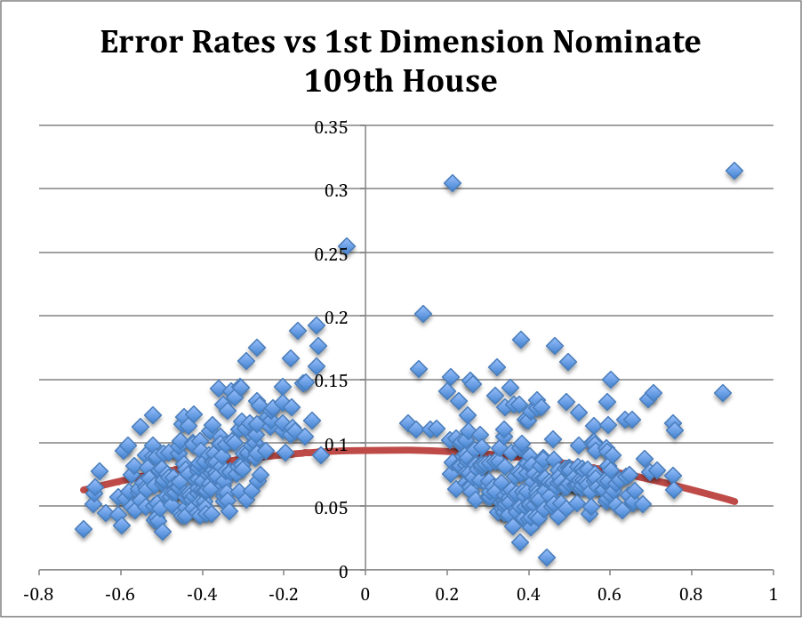
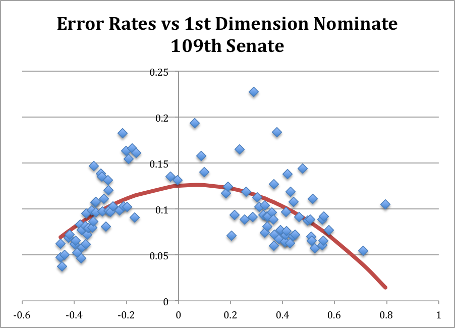
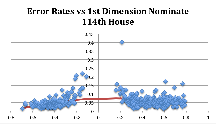
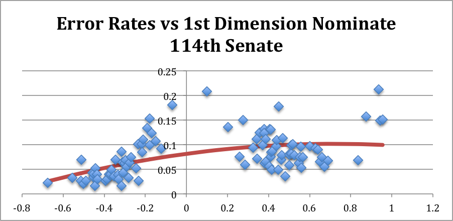
The “Hook”: Consider algorithmic fairness. There’s a well-known result (due to Kleinberg, Mullainathan, and Raghavan, and independently to Chouldechova) showing that two natural fairness criteria — error-rate balance and predictive parity — are generally incompatible when different groups have different base rates of the behavior the algorithm is trying to predict. This is, in its structure, an impossibility theorem of the same species as the ones we’ve been discussing: you can’t have everything you want, simultaneously, within the system.

Now, in some recent work that Maggie Penn and I have been doing, we noticed something. The classical impossibility results hold behavior fixed — they assume that people’s base rates of compliance (or recidivism, or default, or whatever the algorithm is classifying) are just facts about the world, not choices that respond to incentives.

But of course they are choices that respond to incentives, and in particular they respond to the stakes of classification — the severity of the fine, the length of the sentence, the terms of the loan. Once you recognize that base rates are endogenous — that they’re equilibrium objects shaped by the algorithm and its consequences — an escape route from the impossibility opens up. You can simultaneously achieve error-rate balance and predictive parity by adjusting the stakes of classification to induce equal base rates across groups.

Cool, …problem solved, right?

Not quite. Here comes the conservation law. The statistical impossibility disappears, but it migrates: achieving both fairness criteria requires that identical classification decisions carry different consequences for different groups. You’ve moved the inequality from the distribution of algorithmic outcomes to the severity of consequences attached to those outcomes. The impossibility doesn’t vanish. It changes address. And it gets worse — in a way that connects directly to the penalty-ceiling problem. In some cases, equalizing base rates under equal stakes requires penalizing compliance — effectively setting negative incentives that suppress the behavior the system is supposed to encourage.

That’s the fairness equivalent of flattening the penalty gradient between assault and murder. You’ve “equalized” the treatment, but you’ve destroyed the incentive structure that was generating the behavior you wanted. The gap migrates, again, from one form of unfairness to another.

I think this is a general feature of any system that tries to regulate strategic behavior. The gap between what the rules intend and what agents can do is not a deficiency of any particular set of rules. It is a structural property of the relationship between rules and the strategic agents who inhabit them. Fix it here, and it appears there. Close this loophole, and you open that one. The impossibility is conserved.

A Provocation for Next Time

So if the impossibility always migrates — if every fix to a rule system creates new gaps somewhere else — then what does this mean for the biggest, most complicated “games” we play? What does it mean for institutions, bureaucracies, governments? It means, I’ll argue, that every well-functioning institution is riddled with informal patches — norms, workarounds, conventions, and practices that exist precisely to handle the cases the formal rules can’t reach.

These patches are the institution’s solution to the migration problem: every time a gap was discovered, someone — a bureaucrat, a judge, a middle manager — found a way to cover it, and that patch became part of the operating system. The institution looks messy from the outside because it is messy. It has to be. The formal rules can’t do the job alone, and the patches are where the real work happens. And it means that anyone who looks at those patches and sees only waste, inefficiency, or evidence of a “deep state” is making a very specific error: they’re assuming the game is complete, when we just showed it can’t be.

They’re treating the messiness as a bug, when it is — often, not always, but far more often than reformers tend to appreciate — a feature. There’s also, I think, a deeper thread here about information — about the fact that rules governing who knows what, and who must disclose what to whom, are a particularly fragile species of rule. Poker understands this; the NFL tried and largely failed; and some of our most important legal infrastructure (think §6103) exists precisely at this fault line. But all of that is for next time. (Ed: Oh, you’ll be back…like in 2016? Sheesh.)

For Now, I Leave You with This

In the 1983 film WarGames, a military supercomputer called the WOPR is tasked with simulating global thermonuclear war. It plays every possible scenario — every first strike, every retaliation, every escalation — searching for one that ends in victory. It finds none. After cycling through the entire game tree, it arrives at a conclusion: “A strange game. The only winning move is not to play.” (Ed: I could make a joke about your blog, but I think you already see it, dammit.)

The WOPR, in other words, did what the trilemma says can’t be done: it verified, from within the game, that the game has no self-enforcing solution. It searched the space, hit every penalty ceiling, found every flat region at the top, discovered that every “winning” move triggers a retaliation that migrates the problem somewhere worse — and concluded that the game is, in our terms, formally incomplete.

There is no outcome the rules can assign to “global thermonuclear war” that makes initiating it incentive-incompatible (Ed: Thank goodness, …right?), because the penalty structure maxes out at “everybody dies,” and at that ceiling, the marginal cost of escalation is zero. Of course, the WOPR had an advantage we don’t: it could search the entire game tree. For the rest of us — playing games whose rules we can’t fully verify, in institutions whose patches we can’t fully see, against opponents whose strategies we can’t fully anticipate — the only honest starting point is to admit that the game is bigger than its rules. With that, I leave with one (dated, but memorable, and timeless) question: “Shall we play a game?”

1. He didn’t inform me of this, but my friend and coauthor Tom Clark essentially encouraged me to write this up some months ago. ↩︎
2. Note the “subtle shift” here: I moved from “basketball” to “basketball as governed by” (or, to quote James Scott’s awesome work: “made legible by” a specific institution that, ahem, “provides basketball to the public for their enjoyment and remuneration.” ↩︎
3. And here’s an additional wrinkle: the NBA’s rules say that no team may be reduced below five players. If a player fouls out (six personal fouls), but there are no eligible substitutes, that player stays in the game and is charged with a personal foul, a team foul, and a technical foul for each subsequent infraction. So ejections are actually the only mechanism that can force a team below five — which means our strangler has, in addition to getting himself tossed, potentially inflicted a roster-count penalty on his own team. But note: this is the same roster-count penalty he’d have inflicted with a garden-variety Flagrant 2 for an overly aggressive screen. The punishment doesn’t scale with the severity of the act. (And even the “stay in the game with a technical” rule is itself manipulable. If your player just picked up his sixth foul with 30 seconds left in a close game, is the team better off keeping him on the court — where every subsequent foul triggers another technical free throw for the opponent — or just… letting him leave and playing 4-on-5? The rule was designed to protect teams from being shorthanded. But in the right circumstances, the “protection” costs more than the problem it solves. We’ll see this pattern again.) ↩︎
4. Speaking of “ceilings,” I am tempted to ask what Naismith would have thought of physical “ceilings” in laying out the initial rules of basketball. Don’t know if he was a physicist or even that “sophisticatedly rational” to think about it, but I would suppose that he would have eventually agreed that “having a ceiling over the game” where you throw a ball up high to avoid defenders’ hands would “only complicate” the eventual performance (and adjudication) of his new game. This makes think of both XFL and Arena Football: both are fun, partly because they borrowed some of the elements of an “already legible sport” (i.e., American Football) and “slightly modified” the nature of the constraints in that sport…) ↩︎
5. For simplicity, let’s just think about “games” where there can be no more than one winner. That a lot looser than “zero-sum”in a formal sense, but with two players, it’s basically without loss of interesting generality (and, yes, I am an American, and I do (in my heart) think “ties are boring.” But that’s maybe why, or because, I find faculty meetings generally unsatisfying. There’s a lot in there, I know.) ↩︎
6. I think the idea that “kingmaking” is a recognized verb should make all of us think more about the nature of language in both analytical and sociological terms. ↩︎
7. I say “the rules” have “handed you” this to differentiate it from very real, “expressive” feelings of guilt or failure from being labeled “a loser.” Just ask our president DJT. The only thing he hates more than rules is being (or, it seems, being associated with) “a loser.” ↩︎

It’s been almost ten years since I’ve written here. The last time I posted, Donald Trump had just clinched the GOP nomination, his Banzhaf power index had hit 1.0, and I was calculating the proportion of his campaign contributions that were unitemized.¹ That was June 2016. I stopped writing because the general election demanded a firehose of commentary I didn’t have the time or the stomach for, and the opportunity cost of blogging versus finishing actual research was getting untenable.

A lot has happened. Some of the people who used to read this blog — colleagues, friends, people I admired — aren’t here anymore. I won’t make a list, because that isn’t what this space is for, but I’ll say that their absence is felt, and that part of what brings me back is the sense that the kind of work this blog tries to do — taking the math seriously, taking the politics seriously, and refusing to pretend you can do one without the other — matters more now than it did when I left.

For those who are new: this is a blog about the math of politics, which is a thing that exists whether or not anyone writes about it. The tagline is three implies chaos, which is a reference to the fact that collective decision-making with three or more alternatives is, under very general conditions, a mess.² I’m a political scientist at Emory. I use formal models — game theory, mechanism design, social choice — to study how institutions shape behavior. And I write here when something in the news is so perfectly illuminated by the theory that I can’t not.

Today a federal judge ruled that the IRS violated federal law approximately 42,695 times, and I have a model for that. Let’s go.

---

NA NA

Last April, Treasury Secretary Bessent and DHS Secretary Noem signed a memorandum of understanding allowing ICE to submit names and addresses to the IRS for cross-verification against tax records. ICE submitted 1.28 million names. The IRS returned roughly 47,000 matches. The acting IRS commissioner resigned over the agreement. And Judge Colleen Kollar-Kotelly, reviewing the IRS’s own chief risk officer’s declaration, found that in the vast majority of those 47,000 cases, ICE hadn’t even provided a valid address for the person it was looking for — as required by the Internal Revenue Code. The address fields contained entries like “Failed to Provide,” “Unknown Address,” or simply “NA NA.”³

NA NA.

That’s what ICE typed into the field that was supposed to ensure the government could only access tax records for individuals it had already specifically identified. And the IRS said: close enough.

Now, the obvious story here — the one you’ll get from the news — is about a legal violation and an institutional failure. And that story is correct. But there’s a deeper story, one that requires thinking about what classification systems do to the populations they classify. Because the address field in the §6103 request wasn’t just a data element. It was a constraint — a design specification that determined what kind of system the IRS-ICE pipeline would be. With the address requirement enforced, the system is a targeted lookup: you ask about a specific person you’ve already identified, and the IRS confirms or denies. With the address requirement collapsed — with “NA NA” treated as a valid input — the system becomes a dragnet. Same code, same database, same agencies. But a fundamentally different machine, operating under fundamentally different logic, with fundamentally different consequences for the people inside it.

I want to talk about those consequences. Specifically, I want to talk about what happens to the population being classified when the classifier changes.

---

Filing Taxes as a Strategic Choice

Here’s the setup. If you’ve read the work Maggie Penn and I have been doing on classification algorithms, this will look familiar.⁴

Undocumented immigrants in the United States pay taxes. They do this using Individual Taxpayer Identification Numbers (ITINs), which the IRS issues specifically to people who have tax obligations but aren’t eligible for Social Security numbers. Filing is not optional — the legal obligation exists regardless of immigration status. But the compliance rate — how many people actually file — has historically been sustained by a critical institutional feature: a firewall between tax data and immigration enforcement. Section 6103 of the Internal Revenue Code strictly prohibits the IRS from sharing taxpayer information with other agencies except under narrow, court-supervised conditions.

The firewall is what made tax filing a safe act. Filing carried a compliance benefit — potential refunds, building a record for future status adjustment, staying on the right side of the IRS — and essentially zero enforcement cost. The tax system observed you, but the immigration system couldn’t see what the tax system saw.⁵ To put it in terms we’ll use throughout: the classifier’s expected responsiveness was zero.⁶ When the classifier is null, people make their filing decision based solely on the intrinsic costs and benefits of compliance. Call that sincere behavior.

The MOU blew a hole in that firewall. After the MOU, filing generates a signal — the tax record, including your address — that feeds directly into an enforcement match. Before the breach, the only classifier that mattered was the IRS’s own enforcement system, and that system rewarded filing: if you complied, you reduced your probability of audit, penalty, and all the administrative misery that follows from the IRS noticing you didn’t file. The reward was real, the classifier was responsive to compliance, and the equilibrium worked.

The MOU layered a second classifier on top — the ICE match — and this one runs in the opposite direction. Filing still reduces your IRS enforcement risk, but it now increases your immigration enforcement risk, because filing is what generates the data that feeds the match. For citizens and legal residents, the second classifier is irrelevant — they face no immigration enforcement cost, so the net calculus doesn’t change. For undocumented immigrants, the second classifier dominates. The expected cost of filing went up, and for many people it went up enough to swamp the expected benefit.

The equilibrium compliance rate in the model is

$$\pi_F(\delta, \phi, r) = F(r \cdot \rho(\delta, \phi))$$

where $r$ captures the net stakes of being classified and $\rho$ captures how much the classifier’s decision depends on the individual’s behavior.⁶ When the firewall was intact, the net reward to filing was positive — the IRS classifier rewarded compliance, and the immigration system couldn’t see you. When the firewall broke, the net reward dropped, in some cases below zero, and the filing rate dropped with it. Not because the legal obligation changed. Not because the refund got smaller. Because the classifier changed, and people responded.

This is a point that’s worth pausing on, because it’s general and it’s important: classification systems do not passively observe the world. They reshape it. A credit-scoring algorithm changes how people use credit. An auditing algorithm changes how people report income. A policing algorithm changes where people walk. The instrument and the thing being measured are not independent of each other, and any analysis that treats them as independent will be wrong in a specific, predictable direction: it will overestimate the accuracy of the system and underestimate its behavioral effects.

Think of two cities, each with a system for issuing speeding tickets. One city’s algorithm is designed to ticket speeders — it cares about accuracy. The other city’s algorithm is designed to generate revenue — it tickets indiscriminately. Drivers in the accuracy-motivated city slow down, because compliance is rewarded. Drivers in the revenue-motivated city don’t bother, because ticketing has nothing to do with their behavior. Same roads, same drivers, same speed limits. Different classifiers, different equilibria. The classifier doesn’t just measure the city — it makes the city.⁷

---

The Death Spiral

This is where it gets interesting. And by “interesting” I mean “bad.”

The people most likely to be correctly identified by the IRS-ICE match are those with stable addresses who file consistently and accurately. These are, almost by definition, the most compliant members of the undocumented population — the ones who’ve been following the rules, building a paper trail, doing exactly what the system told them to do. They’re also the ones with the most to lose from enforcement, because they’ve given the system the most data about themselves.

These are the first people who stop filing.

Judge Talwani flagged this directly. Community organizations that provide tax assistance to immigrants can’t advise their members to stop filing — that would be encouraging illegal behavior. But they also can’t encourage filing, because filing now triggers enforcement risk. The organizations reported decreased revenue and participation. The chilling effect isn’t hypothetical. It’s in the court record.

Now here’s the feedback loop. When the most identifiable filers exit the system, the quality of the remaining data degrades. The match rate goes down. The false positive rate — the probability that a match incorrectly targets a citizen or legal resident — goes up, both because the denominator of correctly matched records shrinks and because ICE is submitting garbage inputs (“NA NA”) that the IRS is accepting anyway. The classifier gets worse at its stated objective precisely because it’s operating.

The system doesn’t just get unfair. It gets worse at its own stated purpose — identifying specific individuals — because the individuals it could most easily identify are exactly the ones who stop showing up.

This is a general property of classification systems with endogenous behavior, and it’s one I think about a lot. When the population being classified can respond to the classifier, the classifier doesn’t observe a fixed distribution. It selects the distribution that’s willing to be observed. And that selection runs in exactly the wrong direction if your goal is accurate identification: the easy cases exit, the hard cases remain, and accuracy deteriorates as a function of the classifier’s own operation. The system eats its own inputs.⁸

---

What the Designer Wants Matters

One of the results Maggie and I are most insistent about is that the objectives of the entity doing the classifying shape the equilibrium in ways that aren’t obvious from the classifier’s structure alone. Two cities with identical data, identical populations, and identical infrastructure but different objectives will design different classifiers, induce different behavior, and produce different social outcomes. The objectives live inside the algorithm, not alongside it.

So: what is DHS trying to do?

The official framing is accuracy-aligned. DHS says the goal is to “identify who is in our country.” That sounds like accuracy maximization: correctly match individuals to their immigration status.

But the implementation tells a different story. An accuracy-maximizing designer needs good inputs — the whole point of the §6103 requirement that ICE provide a valid address is to ensure the system operates on pre-identified individuals, which is a precondition for accurate matching. ICE submitted “NA NA.” They submitted jail addresses without street locations. They submitted 1.28 million names and got 47,000 matches, meaning a 96.3% non-match rate before you even get to the question of whether the matches were accurate.

This doesn’t look like accuracy maximization. It looks like a fishing expedition — a bulk data pull designed to maximize the reach of the enforcement system rather than the precision of individual identifications. In the language of the paper, it looks more like compliance maximization (or its dark inverse: maximizing the chilling effect on a target population) or outright predatory objectives — a system that benefits from inducing non-compliance, because non-compliance makes the targets more vulnerable, not less.⁹

And the distinction between objectives matters formally, because the two produce different classifiers with different welfare properties. An accuracy-maximizing classifier, we show, will push some groups toward compliance and others away — exacerbating behavioral differences between groups even when the data quality is identical across groups. A compliance-maximizing classifier, by contrast, always satisfies what we call aligned incentives: it pushes all groups in the same behavioral direction.

Here, the groups aren’t abstract. They’re citizens, legal residents, and undocumented immigrants, all of whom file taxes, all of whom had their data swept into the same match, and all of whom face different enforcement costs from being identified. The classifier doesn’t distinguish between them at the input stage — it just matches names and addresses. But the behavioral response to the classifier differs radically across groups, because the stakes of being classified differ radically. Citizens face essentially zero enforcement cost from a match. Undocumented immigrants face deportation. The same classifier, applied to the same data, produces wildly different equilibrium behavior in different populations.

That’s not a bug in the implementation. That’s a structural property of classification systems with heterogeneous stakes. And it’s a property that accuracy maximization makes worse, not better.

---

The Commitment Problem

There’s one more piece of the model that’s eerily relevant. We distinguish between designers who can commit to a classification algorithm and designers who are subject to audit — who must classify consistently with Bayes’s rule and their stated objectives. The commitment case is more powerful: a designer who can commit can deliberately misclassify some individuals to manipulate aggregate behavior. The no-commitment case, which we interpret as the effect of auditing or judicial review, strips away this power.

Judge Kollar-Kotelly’s ruling is an audit. She looked at what the IRS actually did — accepted “NA NA” as a valid address, disclosed 42,695 records in violation of the statutory requirement — and said: this doesn’t satisfy the constraints. Judge Talwani’s injunction goes further, blocking enforcement use of the data entirely.

These rulings function exactly as the no-commitment constraint does in the model. They force the classifier to satisfy sequential rationality — to justify each classification decision on its own terms, rather than as part of a bulk strategy to influence population behavior. And the paper tells us what happens when you impose that constraint: the resulting equilibrium satisfies aligned incentives. The designer can no longer push different groups in different behavioral directions.

That’s the fairness argument for judicial review of classification systems, stated formally. It’s not that judges know better than agencies how to design algorithms. It’s that the constraint of having to justify individual decisions prevents the designer from using the algorithm to strategically manipulate aggregate behavior. The cost is accuracy — the no-commitment equilibrium is always weakly less accurate than what the designer could achieve with commitment power. But the benefit is behavioral neutrality across groups, which is a fairness property that accuracy maximization cannot guarantee.¹⁰

---

Where This Goes

The D.C. Circuit will rule on the Kollar-Kotelly injunction. If they uphold it, the no-commitment constraint holds and the data-sharing agreement is dead in its current form. If they reverse — and the Edwards panel’s reasoning from two days ago suggests this is possible — the commitment case reasserts itself, and the behavioral distortions I’ve described become the operating equilibrium.

Meanwhile, the chilling effect is already in motion. People have already stopped filing. Community organizations have already seen decreased participation. The equilibrium is shifting in real time, and it won’t shift back quickly even if the courts ultimately block the agreement, because trust in the firewall is not a switch you can flip. It’s a belief about institutional behavior, and beliefs update slowly after violations — especially violations that occurred 42,695 times.

The tax system was designed as a compliance mechanism: file your returns, pay what you owe, and we won’t use your data against you. That design was a choice. The firewall was a choice. The address requirement in §6103 was a choice. Every one of those choices encoded a judgment about what the system should be for — not just what it should measure, but what kind of behavior it should sustain. The MOU didn’t just breach a legal firewall. It changed the classifier, which changed the equilibrium, which is changing the population, which will change the data, which will change what the classifier can do. The whole thing is a loop, and it’s spinning in exactly the direction the model predicts.

I said I’d be back when something in the news was so perfectly illuminated by the theory that I couldn’t not write about it. This is that. There will be more.¹¹

With that, I leave you with this.

---

^{1. 72.9%, for those keeping score. ↩}

^{2. The phrase is from Li and Yorke’s 1975 paper “Period Three Implies Chaos,” which proved that a continuous map with a periodic point of period 3 has periodic points of every period — plus an uncountable mess of aperiodic orbits. But the tagline does triple duty: Arrow’s theorem, the Gibbard-Satterthwaite theorem, and the McKelvey-Schofield chaos theorem all say that with three or more alternatives, the relationship between individual preferences and collective outcomes becomes fundamentally unstable. Norman Schofield, who proved the general form of the chaos result with Richard McKelvey, was a mentor and colleague to both Maggie Penn and me at Washington University. It was Norman, in a bar in Barcelona, who suggested that Maggie and I write our first book, Social Choice and Legitimacy: The Possibilities of Impossibility, which we dedicated in part to McKelvey. He died in 2018, and he is one of the people I miss when I write here. Three implies chaos. It’s not a bug. It is the central fact of democratic life. ↩}

^{3. The legal landscape is, to use a technical term, a mess. Kollar-Kotelly’s injunction from November is still in effect but under appeal in the D.C. Circuit. Judge Talwani in Massachusetts issued a separate injunction in early February blocking enforcement use of the data. And two days ago, a D.C. Circuit panel declined to enjoin the agreement, reasoning that “last known address” isn’t protected return information under §6103. So you have district courts saying it’s illegal and an appellate panel suggesting it might not be. Three courts, three bins for the same data. If that doesn’t sound like a social choice problem to you, you haven’t been reading this blog long enough. ↩}

^{4. Penn and Patty, “Classification Algorithms and Social Outcomes,” American Journal of Political Science (forthcoming). The formal model and all the results I’m drawing on here are in that paper. What follows is a blog-post-grade application of the framework, not a formal extension of it. But the shoe fits disturbingly well. ↩}

^{5. The firewall wasn’t just a policy preference — it was constitutional load-bearing infrastructure. The government’s power to tax illegal income was established in United States v. Sullivan (1927) and famously applied to convict Al Capone in 1931. But requiring people to report illegal income creates an obvious Fifth Amendment problem: filing becomes compelled self-incrimination. Section 6103 resolved the tension by ensuring tax data stayed behind the wall. With the firewall intact, you could — in principle — write “narco drug lord” in the occupation field of a 1040 and nothing would happen, because the IRS couldn’t share it. The MOU reopened that wound. If filing now feeds ICE, then filing is self-incrimination for undocumented immigrants, and the constitutional bargain that made the whole system work since Sullivan is back in play. Whether anyone is litigating this yet is a question I leave open, but the logical structure is Gödelian: the system simultaneously compels disclosure and punishes the act of disclosing. ↩}

^{6. In the model, expected responsiveness is $\rho(\delta, \phi) = (\delta_1 + \delta_0 – 1)(2\phi – 1)$, where $\delta_1$ and $\delta_0$ are the probabilities that the classifier’s decision matches the signal for compliers and non-compliers respectively, and $\phi$ is signal accuracy. A null classifier has $\rho = 0$: the probability of being targeted is the same regardless of whether you file. The §6103 firewall enforced nullity by severing the link between the signal (tax record) and the decision (enforcement action). ↩}

^{7. This example is from the paper, but it’s the kind of thing that should be folklore by now. It isn’t, largely because the computer science literature on algorithmic fairness has mostly treated the classified population as fixed. That’s starting to change — see Perdomo et al. (2020) on performative prediction and Hardt et al. (2016) on equality of opportunity — but the political science framing, where the designer has objectives and the population has strategic responses, is still underdeveloped. Maggie and I are trying to fix that. ↩}

^{8. There’s also a revenue dimension that shouldn’t be ignored. The IRS estimates that undocumented immigrants pay billions in federal taxes annually. If the filing rate drops — which it will, and which the court record suggests it already is — that’s tax revenue the government doesn’t collect. The classifier was supposed to serve immigration enforcement, but its equilibrium effect includes degrading the tax base. Whether anyone in the administration has done this calculation is an exercise I leave to the reader. ↩}

^{9. Predatory preferences in the model are characterized by a designer whose most-preferred outcome is to not reward an individual who didn’t comply. Think predatory lending: the lender benefits most when the borrower defaults, because the default triggers fees, repossession, or refinancing at worse terms. A designer with predatory preferences over immigration enforcement would want undocumented immigrants to stop filing taxes, because non-filers are more legally precarious, have weaker paper trails, and are easier to deport. Whether this is what DHS actually wants is a question I can’t answer from the model. But the model can tell you what the observable signatures of predatory preferences look like, and “submit NA NA as an address for 1.28 million people” is consistent with the signature. ↩}

^{10. Whether you think that tradeoff is worth it depends on what you think “fairness” means in this context, and reasonable people disagree. But the point is that it is a tradeoff, with formal properties that can be characterized — not a vague gesture at competing values. I have more to say about this, and about how it connects to a set of problems that go well beyond tax data. But that will have to wait for another post. Or, you know, the book. ↩}

^{11. Next up: the Supreme Court just handed us a game-theoretic goldmine, and three implies chaos. Stay tuned. ↩}

Much has been made today of Donald Trump’s lackluster fundraising productivity in May. I’m going to pile on here, because his campaign is an absolute fiasco in essentially every sense.

In lieu of a full analysis of what this means in terms of inference and prediction, here are three simple rankings/comparisons.  (For the full read of the data, see here: Bernie, Hillary, Trump.)

Total contributions, through the entire cycle through May:

1. Bernie: $224 Million.
2. Hillary: $207 Million.
3. Donald: $17 Million.

Candidates can loan money to their own campaign (meaning they can use campaign contributions to pay themselves back):

1. Donald: $45 Million.
2. Hillary: $0.
3. Bernie: $0.

Third, donations to federal campaigns fall into two categories: itemized and unitemized.  Itemized donations are those that, in sum, for an individual, exceed $200.  Unitemized are those that sum to less than $200 for the donor.

With that said, the proportion of donations that are unitemized to date for each candidate:

1. Donald: 72.9%
2. Bernie: 59.0%
3. Hillary: 21.6%

What does this indicate?

First, Bernie and Hillary are vastly outperforming Trump in terms of raising money.  VASTLY. There’s a bit of chicken and egg here, but the simple fact is that raising money requires a ground operation, and the data confirms observation that Hillary and Bernie have such operations in place, and Trump—well, not so much.

Second, Donald Trump is actually self-financing his campgin on the idea that he will get sufficient contributions to pay himself back.  Hillary and Bernie are not doing so.

Third, Hillary’s contributions are coming from “big” donors much more than are Donald’s (limited) contributions or Bernie’s (significant) contributions.  For Bernie, this makes sense: he is appealing to a swath of the US electorate that doesn’t generally have the wherewithal to donate $200 to a political campaign.

For Trump, maybe the same argument applies…Don’t know.  It’s just a very large ratio of unitemized contributions.  I’ll leave it there.

With this, and in light of the absolutely shameful failure of the Senate to undertake serious efforts at preventing gun violence yesterday, I leave you with this.

The Republican Party is in crisis. This year’s presidential campaign is arguably evidence enough for this conclusion, but it is important to remember that there are really (at least) two “Republican Parties”: one composed of voters and another composed of Members of Congress.

A split in the broader GOP is troublesome for Republican elites because, among other things, it complicates the quest for the White House, which might also cause significant problems for Republican Members seeking reelection. But splits in the broader party do not necessarily affect governing. A split in the “party in Congress,” however, can greatly complicate governing. Indeed, one might argue that the beginnings of such a split caused the downfall of former Speaker Boehner, the government shutdown of 2013, and the near-shutdown of 2015.

As Keith Poole eloquently notes, the potential split in the GOP appears eerily similar to the collapse of the Whig Party in the early 1850s (the last time a major party split occurred in the United States). A key difference between the current Congress and those in the 1850s is the lack of a “second dimension” of roll call voting. Without going into the weeds too much, what this means is that there is no systematic splitting of the Republican party on a repeatedly revisited issue. In the 1850s, that issue was slavery (specifically how it would be dealt with as the nation admitted new states).

Because of this, our roll call-based estimates of Members’ ideologies essentially place all members on a single, left-right dimension. This implies that, for most contested roll call votes, most of the Republicans vote one way and most of the Democrats vote the other. The figure below, which displays the proportion of roll call votes in each Congress and chamber that pitted a majority of one party against a majority of the other, illustrates how this has become increasingly the case.

Of note in the figure are two things. The first is the overall increase in party line voting since the civil rights era. Party line voting was rare during this era in part because the Republican party controlled relatively few seats in either chamber and, relatedly, because the Democratic party often split on civil rights legislation, with Southern Democrats relatively frequently voting with Republicans. As the South “realigned,” beginning in earnest with the 1980 election, the parties became more clearly sorted and party line voting became more common: with civil rights legislation largely off the table, fewer and fewer votes split either party.

The second thing to note is that party line voting dropped precipitously in 1997 (the first Congress of Bill Clinton’s second term), rose during George W Bush’s presidency, and unevenly surged during Obama’s first 3 Congresses. Thus, “partisan voting” is definitely not on the decline in recent years.  This is important for many reasons, but for our purposes it is important because it implies that the nature of “partisan warfare” has not qualitatively changed in terms of the structure of roll call voting, writ large.

Unpredictability and Ideology

Given a Member’s estimated ideology (“ideal point”), we can predict how that member should have voted on each roll call vote. (I am omitting some details.) Using this and the actual votes, we can calculate how many times each Member’s vote was “mispredicted” by the estimated ideal point.

In a nutshell, these are situations in which most of the other Members who have similar ideological voting records voted (say) “Yea,” members on the other side of the ideological spectrum voted “Nay” and the member in question voted “Nay.” For example, if all of the Democrats voted “Nay” on some roll call, and all of the Republicans other than Ted Cruz voted Yea, then Senator Cruz’s vote would be mispredicted by Cruz’s estimated ideal point (which is the most conservative among the current Senate).

Typically, this misprediction, or “error” rate is higher for Members who are (estimated to be) ideological moderates. This is for several reasons. First, if a member is simply voting randomly, then he or she would be estimated to be a moderate. Second, and more substantively, if a member is actually moderate, then his or her vote is more likely to be determined by non-ideological factors because his or her ideological preferences are relatively weaker than for someone who is ideologically extreme.

In any event, the figures below illustrate the House and Senate for a “typical” recent Congress, the 109^th Congress (2005-6). In the 109^th both chambers of Congress were controlled by the Republican Party, following the reelection of George W. Bush. In both figures, the horizontal axis is the estimated ideology so dots on the left represent liberals and dots on the right represent conservative), and the vertical axis is the proportion of votes cast by that member that were mispredicted by his or her estimated ideology. Each figure includes an estimated quadratic equation for “expected error rate.”[1]

 

In both figures, with one notable exception in the 109^th House (Ron Paul (R, TX), Senator Rand Paul’s father), bear out the general tendency for moderates to have higher error rates than “strong” liberals and conservatives. [2]

What About Today? Let’s turn to the 114^th Congress (through March 2016). Looking first at the House, the pattern from the 109^th is still present.[3] Moderates are characterized by higher error rates than strong liberals or conservatives.

In the 114^th Senate (through March 2016), however, the picture is qualitatively and statistically different:
In particular, the Republican party has generally higher error rates than does the Democratic party.[5] This indicates that Republican Senators have been more likely to vote against their party than have been Democratic Senators or, more substantively, the internal ideological structure of the Republican party in the Senate has played a smaller role in determining how GOP Senators have voted in this Congress.

Who’s Being Unpredictable?

Consider the list of the 15 Senators with the highest error rates:

Name	State	Error Rate	Party	Conservative Rank
PAUL	Kentucky	21.2%	GOP	3rd
COLLINS	Maine	20.8%	GOP	54th
MANCHIN	West Virginia	18.1%	Dem	55th
HELLER	Nevada	17.7%	GOP	29th
FLAKE	Arizona	15.7%	GOP	4th
KING	Maine	15.3%	Independent	60th
CRUZ	Texas	15.1%	GOP	1st
KIRK	Illinois	15.0%	GOP	51st
LEE	Utah	14.9%	GOP	2nd
MURKOWSKI	Alaska	13.6%	GOP	53rd
NELSON	Florida	13.4%	Dem	61st
PORTMAN	Ohio	13.2%	GOP	44th
MORAN	Kansas	13.1%	GOP	38th
MCCONNELL	Kentucky	13.0%	GOP	37th
AYOTTE	New Hampshire	12.4%	GOP	46th
HEITKAMP	North Dakota	12.4%	Dem	58th
MCCAIN	Arizona	12.4%	GOP	43rd
GARDNER	Colorado	11.3%	GOP	26th
GRASSLEY	Iowa	11.1%	GOP	48th
CORKER	Tennessee	11.1%	GOP	41st

Tellingly, the four most conservative Senators have incredibly high error rates (and two of these (Paul and Cruz) made serious runs for the GOP presidential nomination). The rest of the list is dominated by Republicans. The four non-GOP Senators are in fairly conservative states (with Maine being an unusual case).[6]

Hindsight and looking back… I don’t have time to get into the weeds even more with this at this moment. For now, I just wanted to point out that voting in the current Senate is unusual: Republicans are breaking with their party more often than are Democrats, and a handful of “extreme” conservatives are breaking with the party at incredibly (indeed, historically) high rates. To quickly see the recent past, consider the 113^th Congress:

In the last Congress, Republicans were already breaking with their party at qualitatively higher rates than were their Democratic counterparts, but there was no real analogue to the cluster of 4 extremely conservative Senators who have been mispredicted so strongly in the 114^th Congress. One of those 4—Senator Flake (R, AZ) was a newly-arrived freshman Senator in the 113^th Congress and has continued to be difficult to predict in his second Congress.

What does it mean? 

In line with both Keith Poole’s conclusion that the GOP shows significant signs of breaking up and the recent revolt among the GOP members in the House (where agenda setting is much more tightly centralized), I think what is happening is that (some of) the “estimated as conservative” wing of the GOP in the Senate is increasingly breaking party lines in pursuit of issues that are not being addressed by the chamber. Qualitative examples of such behavior are seen in the recurrent obstructionism among the “Tea Party wing” of the Republican party. (For example, see my theoretical work on this type of behavior and its electoral origins.) This rhetoric has also flared in the race for (both parties’) presidential nominations.

In line with this, of course, is the fact that the GOP has a disproportionately large number of Senators up for reelection in 2016. I haven’t had time to go through and compare the list of highly mispredicted Senators (please feel free to do so and email me about it!), but my hunch is that a bunch of “in-cycle” Senators are on that list.

For now, though, I leave you with this and this.

________________

 

[1] The quadratic term is significant (and obviously negative) in both chambers, as typical.

[2] The other Members with similarly high error rates in the House are Gene Taylor (D, MS), who would go on to be defeated 4 years later in the 2010 election, and Walter Jones (R, NC), who will show up again below: both were considered “mavericks” and were, as a result, estimated as being relatively moderate in ideological terms. In the Senate, the three highest error rates were (in order) Senator Mike DeWine (R, OH), who would be defeated in the 2006 midterm election by Sherrod Brown, Senator Arlen Specter (R, PA), a moderate Republican, and Senator John McCain (R, AZ).

[3] The quadratic term for the estimation of the relationship between estimated ideal point and error rate is again significant and of course negative.

[4] The quadratic term in this case is still negative, but no longer statistically significant. The linear term is positive, of course, and statistically significant.

[5] As is common in recent Congresses, there is no overlap between the parties’ ideological estimates so far this Congress: Senator Joe Manchin (D, WV) is the most conservative Democratic Senator, and Senator Susan Collins (R, ME) is the most liberal Republican Senator, but Senator Collins is estimated as being more conservative than Senator Manchin.

[6] Mitch McConnell is on this list for procedural reasons: he frequently votes “with” the Democrats on cloture motions when it is clear that cloture will fail, so as to reserve the right to motion to reconsider the vote in the future.

 

This is a guest post by David Epstein. 

Picture this: you are on a committee to hire a new CEO for a large, multinational firm. There are a number of qualified candidates, you are told, each of whom has many years of experience in the relevant field, and then you are handed a background folder on each of them. In the folder you find detailed statements of what they would like to do with the company if they are hired.

So far so good, but when it comes to the candidates’ histories, the folder talks only about their deep formative experiences from when they were children, along with some amusing anecdotes from their lives over the past few years. Nowhere, though, does it tell you how these candidates have actually performed in their professional careers. Have they been CEO’s before? If so, how did their companies do? What projects have they tackled in the past, and what were the outcomes? All excellent questions, but nothing in the files provides any answers.

This is the situation voters find themselves in every four years when choosing a president. They are told what policies the candidates promise to enact if elected, sometimes with an evaluation of how realistic and/or desirable those policies would be. But nowhere, for the most part, are they given the candidates’ backgrounds in jobs similar to the one they are running for. (An outstanding exception to this rule is Vox’s review of Marco Rubio’s tenure as Speaker of the Florida House of Representatives.)

The Task Ahead

Here, I will begin to remedy this gap by comparing the legislative records of the four candidates who have spent time in the Senate: Sanders, Clinton, Rubio and Cruz. Sanders has proposed a “revolutionary” set of reforms; how likely is he to be able to make them into policy? Clinton spent twice as long as a senator from New York than as Secretary of State, but somehow that chapter in her political history is rarely spoken about. Rubio and Cruz are newer to the Senate, Rubio more of an establishment legislative figure (at least at first), and Cruz more clearly ideological. Do either of them have histories of getting their policies passed? And yes, it’s true – Rubio and Cruz have now dropped out of the race. But a) they might still be on the ballot as VP candidates, and b) it is interesting to compare them with the Democrats, as explained below.

Now, no one set of measures can completely capture how well a legislator does their job. I’ll be examining statistics having to do with proposing, voting on, and passing legislation, which might be considered legislators’ core activities. But members of Congress also must spend time doing constituency service, sitting on committees and subcommittees, appearing in the media, and more. And, of course, what of the candidates who were executives (governors) previously — how should we measure their performance? This analysis isn’t meant to be the final word on the subject; rather, it should provide some interesting material to consider and, hopefully, open a wider discussion on assessing candidates’ qualifications for the presidency.

TL;DR: Clinton comes out looking good in terms of effectiveness and bipartisan cooperation, and Rubio does surprisingly well for his first term, sliding down after that. Sanders had a burst of activity from 2013-14, but his years before and after that aren’t very impressive. Cruz’s brief time in the Senate has been almost completely unencumbered by working to pass actual legislation.

Left-Right Voting Records

Let’s start by looking at how liberal/conservative the candidates’ voting patterns were while in office. Political scientists have developed a scale for measuring the left-right dimension of voting, called the Nominate score. I ranked these scores by Congress, with 1 indicating the senator with the most liberal voting record, and 100 being the most conservative. [NB: Each Congress lasts two years, with the 1st going from 1789-1790, and so on from there. For our purposes, the relevant Congresses stretch from the 107th (2001-02) to the current 114th Congress (2015-16). Since the 114th isn’t over yet, its statistics should be correspondingly discounted relative to the others.]

As shown in the table below, the four candidates form almost perfectly symmetric mirror images of each other. Clinton was around number 15 during her four terms in the Senate, while Rubio was 85. So each of them, despite being tagged as the “establishment” or “moderate” candidates in the primaries, was each more extreme than the average member of their own parties. That is, Clinton voted in a reliably liberal direction, even more so than the majority of her Democratic colleagues, while the same holds true for Rubio vis-à-vis the Republican senators.

Congress	State	Name	Rank
107	NEW YORK	CLINTON	14
108	NEW YORK	CLINTON	15
109	NEW YORK	CLINTON	13
110	VERMONT	SANDERS	1
110	NEW YORK	CLINTON	15
111	VERMONT	SANDERS	1
112	VERMONT	SANDERS	1
112	FLORIDA	RUBIO	85
113	VERMONT	SANDERS	1
113	FLORIDA	RUBIO	86
113	TEXAS	CRUZ	100

The Candidates, Ranked by the “Liberalness” of their Senate Voting
(1: Most Liberal, 100: Most Conservative)

Sanders and Cruz also form a perfect pair of antipodes. Sanders had the most liberal voting record for each of his terms, while Cruz was the most conservative. As a note: the only time that a party’s nominee had the most extreme voting record in their party was George McGovern in 1972 –- draw your own conclusions.

The symmetry is broken, however, when you consider the states the candidates represent(ed). Vermont is by many opinion poll measures the most liberal state in the country, and Clinton’s rank almost perfectly reflects New York’s relative position as well. Cruz and Rubio, on the other hand, have voting records considerably more conservative than Texas (number 33 out of 50 in conservative opinions of its voters) or Florida (number 23 out of 50) residents, respectively.

Bill Passage

Voting analysis can give us clues to the kind of policies a president might pursue in office. But can they get legislation passed? The next two figures show the number of bills and amendments introduced by each candidate, and the number of those that eventually passed into law, along with the overall average for each Congress.

Note first that, although the average number of bills introduced has stayed more or less constant over time, the number actually passed has taken a nosedive in recent years. This reflects the increased partisan divisions in Congress, as well as the electorate, that have made Obama’s second term one where policy change may happen via executive actions or rulings in important Supreme Court cases, but rarely via the normal legislative route.

In terms of the various candidates, Clinton was by far the most active in terms of introducing and passing legislation; her totals are significantly above congressional averages for each of her terms in office. This makes sense in terms of her political history: Clinton entered the Senate in 2001 with a lot to prove — she had won just 15 of New York’s 62 counties in her 2000 election victory and wanted to establish herself as a legislator who could get things done. She worked hard, especially pushing programs that benefitted upstate New York’s more rural, agricultural economy, and was rewarded in 2006, winning re-election handily with a majority in 58 counties.

Sanders, on the other hand, has fewer legislative achievements to his name. He had a spurt of activity in the 113th Congress (2013-14), where, perhaps looking forward to his upcoming presidential bid, he introduced 69 measures, four of which passed into law. As noted above, Sanders has consistently represented his state’s liberal voters, but while the policies he has proposed may have been popular at home, in general they have not won sufficient support to be enacted into law.

Cruz and Rubio are about average in terms of measures introduced and below average for number passed. Neither, to date, has a major legislative initiative to their name. But see the next section, for Rubio’s record has more to it than it seems.

Co-Sponsorship

Actually passing policy means getting others to support your positions, and in today’s environment that entails getting members of the opposite party to vote in favor of your proposals, at least every once in a while.

Thus we now turn to analysis of cosponsorship trends. When a bill or amendment is introduced by a member of Congress — making them the “sponsor” of that measure — other members of their chamber can register their support for it by adding themselves as “co-sponsors.”

As the figure below shows, even though Clinton was far ahead of the others in terms of getting her bills passed into law, she did not have an especially high number of cosponsors per bill, on average. Neither did any of the other candidates, with the notable exception of Rubio in his first few Congresses.

As the chart shows, the few measures that he introduced in his first years in office were relatively high-profile, gaining the support of a number of colleagues. However, the efforts produced few results, one example being the immigration reform bill he introduced as a member of the bipartisan “gang of eight” after the 2012 elections. Thus Rubio’s time in the Senate — somewhat similar to his presidential campaign — started out with a flurry of activity but then faded out, as he failed to assemble coalitions to get behind his proposals.

To measure the candidates’ track records of creating bipartisan coalitions, we look at two measures of their ability to attract the support of their colleagues from across the aisle. First, the percent of cosponsors who come from the opposite party. Second, a measure of “cosponsor coverage,” meaning the number of senators who cosponsored at least one measure proposed by the given candidate in the course of a single Congress.

All of the candidates perform a bit below average in the percent of cosponsors from the opposite part, with Clinton and Rubio again doing better than Sanders or Cruz. And in the coverage measure, Clinton is relatively high, with Sanders and Rubio close on her heels (except for the most recent Congress, where Sanders has almost no cosponsors for the measures that he has introduced). Cruz is especially low in coverage, gaining three Democratic supporters in his first term, and four in this, his second term. Of course, Cruz has spent his time in the Senate mainly working to oppose existing policies (via government shutdowns and filibusters) rather than create new ones, so this is not too surprising.

Conclusions

Of course, there has been one other sitting senator — the first since John F. Kennedy in 1960 — elected to the presidency, and that is Obama, who spend four years in the Senate prior to his election in 2008. (Nixon spent two years in the Senate before becoming Eisenhower’s VP, and Lyndon Johnson was a senator when he became Kennedy’s VP.) What would this analysis have said about him?

Obama’s voting record was a tad more conservative than Clinton’s — number 18 on the list compared to her 15 — but he also represented a slightly less liberal state than she did. He proposed an average of 68.5 bills each Congress, which is higher than average, but he only passed a below-average 1.5 bills per Congress. Thus Obama had a lot of ideas about what to do, but didn’t yet have the track record of being able to work with his fellow senators to bring these ideas to fruition.

Interestingly, Obama’s bipartisan measures are all average or above average compared to the other candidates, so while trying to garner support for his bills he was able to work with Republicans fairly well. This would probably have made it even more of a surprise when, once he took office, the Republican party as a whole refused to work with him in any fashion to pass his policy agenda.

The Democratic and Republican Parties each use a weighted voting system to choose their presidential nominees.  This only matters when no candidate has a majority of the delegates, and the details are complicated because the weight a particular candidate has is actually a number of (possibly independent) delegates.  Leaving those details to the side, let’s consider how much Donald Trump’s wins on Tuesday April 26th “mattered.”  The simplest measure of success, for each candidate, is how many additional delegates they each won.  As a result of Tuesday’s primaries, Trump is estimated to have picked up 110 delegates, Senator Cruz is estimated to have picked up 3, and Governor Kasich similarly is estimated to have picked up 5.

A key concept in weighted voting games is that of power.  There are literally countless ways to measure power, but one of the most popular ways is called the Banzhaf index.

If there are total votes, and a candidate “controls” of those votes, the Banzhaf index measures the probability, given the distribution of the other  votes across the other candidates, that the candidate in question will cast the decisive vote: that is, that he or she will have enough votes to pick the winner, given every way the other candidates could cast their ballots. (I’m skipping some details here.  For the interested, the most important detail is that the index presumes that the other candidates will randomly choose how to vote.)

A higher power index implies that the candidate is more likely to determine the outcome. What is key is that the power index for a candidate with votes out of is generally not equal to .  For example, if a candidate has over half of the votes,[1] then that candidate’s Banzhaf index is equal to 1 (and those of all other candidates are equal to zero, and we’ll see that come up again below), because that candidate will always cast the decisive vote.

So, back to Tuesday.  Here is the breakdown of how the GOP candidates’ delegates translated into “Banzhaf power” before Tuesday’s primaries.

Candidate	Donald Trump	Ted Cruz	John Kasich	Marco Rubio	Ben Carson	Jeb Bush	Carly Fiorina	Rand Paul	Mike Huckabee	Total
Delegates	846 (48.85%)	548 (31.64%)	149 (8.6%)	173 (9.99%)	9 (0.52%)	4 (0.23%)	1 (0.06%)	1 (0.06%)	1 (0.06%)	1,732
Banzhaf Power	0.5	0.1667	0.1667	0.1667	0.1667	0	0	0	0

Going into Tuesday’s primaries, Trump held just under majority of the delegates and held exactly half of the power.  More interesting in this comparison is that Marco Rubio’s power was still significant: in fact, equal to the individual powers of Kasich and Cruz.

Even though Rubio and Kasich each had less than a third of Cruz’s delegates, their voting power as of Monday was equal to Cruz’s. This is due to the fact that Rubio, Kasich, and Cruz could defeat Trump if and only their delegates voted together, regardless of how the other delegate-controlling candidates had their candidates vote.  In other words, Carson, Bush, Fiorina, Paul, and Huckabee truly had—as of Monday (and today)—no bargaining power at a contested convention.

However, after Tuesday’s results, the following happened:

Candidates	Donald Trump	Ted Cruz	John Kasich	Marco Rubio	Ben Carson	Jeb Bush	Carly Fiorina	Rand Paul	Mike Huckabee	Total
Delegates	956 (51.68%)	551 (29.78%)	154 (8.32%)	173 (9.35%)	9 (0.49%)	4 (0.22%)	1 (0.05%)	1 (0.05%)	1 (0.05%)	1,850
Banzhaf Power	1	0	0	0	0	0	0	0	0

By securing a majority of the delegates allocated so far, Trump’s power jumped from 0.5 to 1 and all of his opponents’ powers dropped to zero.  If the convention occurred today, they would be powerless to stop Trump.

Now, suppose that the candidates had votes equal to the actual votes (rather than delegates) they receive.  If the convention were held today under such rules, this would result in the following:

Candidates	Donald Trump	Ted Cruz	John Kasich	Marco Rubio	Ben Carson	Jeb Bush	Jim Gilmore	Chris Christie	Carly Fiorina	Rand Paul	Mike Huckabee	Rick Santorum	Total
Popular Votes	10,121,996 (39.65%)	6,919,935 (27.10%)	3,677,459 (14.40%)	3,490,748 (13.67%)	722,400 (2.83%)	270,430 (1.06%)	2,901 (0.01%)	55,255 (0.22%)	36,895 (0.14%)	60,587 (0.24%)	49,545 (0.19%)	16,929 (0.07%)	25,530,125
Banzhaf Power	0.5	0.1667	0.1667	0.1667	0	0	0	0	0	0	0	0

If the popular votes were the basis of the GOP nomination and the convention were held today, then the candidates would still have the same “powers” as they did prior to Tuesday’s primaries.  Thus, on Tuesday, we arguably truly witnessed the effect of the “delegate system.”

As a final note, this power calculation clearly indicates something that I think is underappreciated about multicandidate races in majority rule settings.  To break Trump’s lock on the race, it is unimportant which candidate (other than Trump) an “unpledged” delegate decides to support.  Right now, if and only if at least 62 unpledged delegates (and I have no idea how many of them there are left right now) decide to support “other than Trump,” then the Trump’s power drops below.  In addition to (and in line with) the fact that it doesn’t matter how those delegates allocate their support across the other candidates, if 62 such delegates appeared in the hypothetical conference tomorrow in Cleveland, the powers of the candidates would be as follows:

Candidates	Donald Trump	Ted Cruz	John Kasich	Marco Rubio	Ben Carson	Jeb Bush	Carly Fiorina	Rand Paul	Mike Huckabee	Total
Delegates	956 (50%)	613 (32.06%)	154 (8.05%)	173 (9.05%)	9 (0.47%)	4 (0.21%)	1 (0.05%)	1 (0.05%)	1 (0.05%)	1,912
Banzhaf Power	0.97	0.004	0.004	0.004	0.004	0.004	0.004	0.004	0.004

Conclusion. There are two “math of politics” points in here. The first is that votes/delegates are definitely not a one-to-one match: indirect democracy is distinct from direct democracy—it’s always important to remember that.  The second, and more “math-y” is that, when people have different numbers of votes, it is not the case that the number of votes a person has is equal to his or her voting power.[2]

With that, I leave you with this.

PS: If you would like (Mathematica) code to calculate the Banzhaf index for this and other situations, email me.

___________

[1] I am assuming for simplicity throughout, in line with the rules of the GOP and Democratic Party, that the collective decision is made by simple majority rule.  One can calculate the Banzhaf index for any supermajority requirement as well.  As the supermajority requirement goes up, the power indices of all candidates with a positive number of votes converge to equality (guaranteed to occur when the decision rule is unanimity).

[2] For a great review of how this is important in the real world, see Grofman and Scarrow (1981), who discuss a real-world use of weighted voting in New York State back in the 1970s.

I posted earlier about truels and how the current GOP nomination approximates one.  In that post, I laid out the basics of the simple truel (i.e., a three person duel), assuming that the three shooters shoot sequentially.  Things can be different when the three shooters shoot simultaneously.[1]  Short version: Trump and Rubio aren’t allies, but game theory suggests they should both attack Cruz, in spite of this.

This is arguably a better model for debates than the sequential version, in which candidates prepare extensively prior to debate, largely in ignorance of the other debaters’ preparations. Leaving that interesting question aside, let’s work this out.  I assume that the truel lasts until only one shooter is left, and that each shooter wants to live, and is otherwise indifferent.  I’ll also assume that the best shooter hits with certainty.[2] The probability that the second-best shooter hits his or her target is 0<p<1 and the probability that the worst shooter hit his or her target is 0<q<p.

When there are two shooters left, each will shoot at the other.  Not interesting, but important, because this implies that the worst shooter wants to shoot at the best shooter in the first round. In the first round, both the second-best and worst shooters shoot at the best shooter.  Either the first best or second best shooter will be dead after this (if the second-best and worst shooter each get to shoot before the first best shooter, but miss, then the second-best shooter will be killed with certainty). There is also a chance that the worst shooter will win in the first round: the best shooter kills the second-best shooter (probability 1/3), and the worst shooter kills the best shooter (probability q<1).

What does this say about the GOP race?  Both Rubio and Trump should be shooting at Cruz.  This is a simplistic model, and it ignores a lot of real-world factors.  But that’s why it’s valuable, from a social science perspective: if (and when) the behaviors of the three campaigns deviate from this behavior, we know that we need to include those other factors.  Until then, you see, in this world there’s two kinds of models, my friend: Those with just enough to capture the logic and those who need to dig for more things to include.  We’ll see if this one needs to dig.

With that, I leave you with this.

____________________

[1]. For simplicity, I will assume that, if two shooters shoot at each other, then one of them, randomly chosen, will “shoot first” and, if he or she kits, kill the other shooter before he or she fires his or her weapon.  Note that, with this assumption, if shooter A knows that shooter B (and only shooter B) is going to shoot at shooter A, then shooter A should definitely shoot at shooter B.

[2]This assumption isn’t as strong as it appears. This is because the truel is already assumed to continue until only one player is left (note that it is impossible for zero shooters to survive, given the tie-breaking assumption).

A truel is a three person duel.  There are lots of ways to play this type of thing, but the basic idea is this: three people must each choose which of the other two to try to kill.  They could shoot simultaneously or in sequence.  The details matter…a lot.  I won’t get into the weeds on this, but let’s think about the GOP race following last night’s Iowa caucus results.  By any reasonable accounting, there are three candidates truly standing: Ted Cruz, Marco Rubio, and Donald Trump.  The three of them took, in approximately equal shares, around 75% of the votes cast in the GOP caucus.

The next event is the New Hampshire primary, and the latest polls (all conducted before the Iowa caucus results) have Trump with a commanding lead and Rubio and Cruz essentially tied for (a distant) second.  So, the stage is set.  Who shoots first?  And at whom?

The truel is a useful thought experiment to worm one’s way into the vagaries of this kind of calculus.  A difference between truels and electoral politics is that the key factor in a standard truel is each combatant’s marksmanship, or the probability that he or she will kill an opponent he or she shoots at.  What we typically measure about a candidate is how many survey respondents support him or her.  For the purposes of this post, let’s equate the two.  Trump is the leader, and Rubio and Cruz are about equal.

A relatively robust finding about truels is that, when the shots are fired sequentially (i.e., the combatants take turns), each combatant should fire at the best marksman, regardless of what the other combatants are doing (this is known as a “dominant strategy” in game theory).  Thus, if we think that the campaigns are essentially taking turns (maybe as somewhat randomly awarded by the vagaries of the news cycle and external events), then both Rubio and Cruz should be “shooting at Trump.”  This is in line with Cruz’s post-caucus speech in Iowa last night.

An oddity of this formulation of the truel is that it is possible that the best marksman is the least likely to survive.  This is true even if the best marksman gets to shoot first.

Is it current, or future, popularity? An alternative measurement of marksmanship, however, is not the current support, but the perceived direction of change in support.  After all, marksmanship is about the ability to kill someone on the next shot.

On this front, Rubio is currently the better marksman: his support in Iowa vastly exceeded expectations, while by many accounts (though not necessarily my own), Trump is the worst marksman.  If one buys this alternative measure, then the smart strategy for both Trump and Cruz is to “aim their guns” at Rubio.  We have a week to see who they each aim at.

Of course, a truel is a simplistic picture of what’s going on in the GOP nomination process. In reality, it is probably better to think that each candidate’s marksmanship depends on his (or her) choice of target.  Evidence suggests that it is harder for Trump to “shoot down” Cruz than it was for him to shoot down Bush.  Maybe I’ll come to that later.  For now, I’m still making sense of Santorum’s strategy of heading to South Carolina. For that matter, I’m trying to make sense of him being called “a candidate for President.”

With that, I leave you with this.

This is math, but it isn’t politics.  This is serious business.  This is the NFL.

The New England Patriots won the coin toss to begin today’s AFC championship game against the Denver Broncos. With that, the Patriots have won 28 out of their last 38 coin tosses. To flip a fair coin 38 times and have (say) “Heads” come up 28 or more times is an astonishingly rare event. Formally, the probability of winning 28 or more times out of 38 tries when using a fair coin is 0.00254882, or a little better than “1 in 400” odds.

But the occurrence of something this unusual is not actually that unusual. This is because of selective attention: we (or, in this case, sports journalists like the Boston Globe‘s Jim McBride) look for unusual things to comment and reflect upon. I decided to see how frequently in a run of 320 coin flips a “window” of 38 coin flips would come up “Heads” 28 or more times. I simulated 10,000 runs of 320 coin flips and then calculated how many of the 283 “windows of 38” in each run contained at least 28 occurrences of “Heads.” (For a similar analysis following McBride’s article, considering 25 game windows, see this nice post by Harrison Chase.)

The result? 441 runs: 4.41%, or a little better than “1 in 25” odds. (Also, note that the result would be doubled if one thinks that we would also be just as quick to notice that the Patriots had lost 28 out of the last 38 coin tosses.)

The distribution of “how many windows of 38” had at least 28 Heads, among those that contained at least one such window, is displayed in the figure below. (I omitted the 9,559 runs in which no such window occurred in order to make the figure more readable.)

 

Accounting for correlation. Inspired partly by Harrison Chase’s post linked to above, I ran a simulation in which 32 teams each “flipped against each other” exactly once (so each team flips 31 times), and looked at the maximum number of flips won by any team. This relaxes the assumption of independence used in both the first simulation and, as noted by Chase, the Harvard Sports Analysis Collective analysis linked to above. I ran this simulation 10,000 times as well. I counted how many times the maximum number of flips won equaled or exceeded 23, which is the number of times the Patriots won in their first 31 games of the current 38 game window (i.e., through their December 6^th, 2015 game against the Eagles).

The result? In 1,641 trials (16.41%), at least one team won the coin flip at least 23 times.

The Effect of Dependence. Intuition suggests that accounting for the lack of independence between teams’ totals decreases the probability of observing runs like the Patriots’. To see the intuition, consider the probability two teams both win their independent coin flips: 25%, and then consider the probability both teams “win” a single coin flip: 0%.

My simulations bear out this intuition, but the effect is bigger than I suspected it would be. Running the same 10,000 simulations assuming independence, at least one team won the coin flip at least 23 times in 2,763 trials (27.63%).

The histograms for the maximum number of wins in each of the 10,000 simulations, first for the “team versus team dependent” case and the second for the “independent across teams” case, are displayed below.

 

Takeaway Message.  Of course, anything that occurs around 5% of the time is not an incredibly common occurrence, but it illustrates that, it’s not that unusual for something unusual to occur. For example, note that the NFC once won the Super Bowl coin toss 14 times in a row (Super Bowls XXXII to XLV), an event that occurs with probability 0.00012207, or a little worse than “1 in 8000” odds. And, of course, we recently saw a coin flip in which the coin didn’t flip.

An empirical matter: somebody should go collect the coin flip data for all teams.  One point here is that looking at one team probably makes this seem more unusual, and the first intuition about the math might suggest that we can simply gaze in awe at how weird this is.  But, upon reflection, we should remember that we often stop to look at weird things without noting exactly how weird they are.

____________________________

Notes.

1. The probability 0.00254882 in the introduction is obtained by calculating the CDF of the Binomial[38,0.5] distribution at 27, and then subtracting this number from 1.  A common mistake (or, at least, made by me at first) is to calculate the Binomial[38,0.5] distribution at 28 and subtract this number from 1. Because the Binomial is an integer valued distribution, that actually gives the probability that a coin would come up Heads at least 29 times. The difference is small, but not negligible, particularly for the point of this post (considering the probability of a pretty rare event occurring in multiple trials).
2. 320 flips is 20 years of regular season games. Not that the streak is constrained to regular season games. I like Chase Harrison’s number (247, the number of games Belichick had coached the Patriots at the time of his post) better, but I didn’t want to re-run the simulations.
3. The probability of this “notable” event is even higher if one thinks that the we would be paying attention to the event even if the Patriots had won only (say) 27 of the last 38 flips.
4. I did the simulations in Mathematica, and the code is available here.

In response to the concerns raised by colleagues (principally and initially in this petition, but see also Chris Blattman’s take and other responses from both sides), I wanted to clarify why I think that delaying implementation of the Journal Editors’ Transparency Statement (JETS) is a poorly thought out goal, one that will differentially disadvantage some scholars, particularly younger, less well-known scholars.

These Standards Are Already Being Implemented. To begin, and reiterate one of the arguments I made here a few days ago, journal editors already have the unilateral discretion to impose the kinds of policies that JETS is calling upon editors to implement. To wit, editors are already implementing policies along these lines. For example, see the submission/replication guidelines of the American Journal of Political Science, American Political Science Review, and the Journal of Politics, to name only three. These three vary in details, but they are consistent with JETS as they stand right now.

It’s Happening Anyway, Let’s Stay In Front of It.  The point is that the JETS implementation is already under way and, indeed, was underway prior to the drafting of JETS. The DA-RT initiative is simply providing a public good: a forum for exactly the conversations that the petition signers seek. (The individuals who have contributed time to the public good that is DA-RT, and their contributions, are described here.)

The Clarifying Quality of Deadlines. The “implementation of JETS” scheduled for January 2016 is best viewed as a moment of public recognition that we as a discipline need to continue the conversations. Editorial policies are not written in stone, after all. Thus I strongly believe that delaying the implementation of JETS will do nothing other than further muddy the waters for scholars. JETS is about recognizing and shepherding the movement towards more coherent and uniform procedures to increase the transparency of social science research. Delaying it will place scholars, particularly junior and less well-known scholars, at a disadvantage. This is because implementation of the JETS will give all scholars firmer ground to stand on when seeking clarification of the details of a journal’s replication and transparency requirements.

Clear Policies Level the Playing Field and Make Editors (more) Accountable. Furthermore, scholars will be able to publicly compare and contrast these procedures, allowing more judicious selection of research design, early preparation of justifications for requests for exemptions, and finally, a counterpoint for an editorial decision that is inconsistent with the standards of peer outlets. That is, if journal X decides that one’s research is sufficiently transparent and then journal Y decides otherwise, the transparency of those journals’ standards—which JETS aims to ensure are publicly available—will ensure that the journals’ standards are fair game for comparison and debate. This is the type of conversation sought by many of the petition signers I have spoken with. Implementation of JETS will push this conversation forward, whereas delay will simply retain the status quo of an incoherent bundle of idiosyncratic policies.

Will The Sun Rise on January 15, 2016? It is important to keep in mind that the implementation of the JETS statement will in most cases result in no new policy: journal editors have been setting and fine-tuning standards like these for decades. Rather, implementing JETS binds editors—like myself—more closely to the sought-after conversations about how best to achieve transparency in the various subfields and with respect to the various methodologies of our discipline.

In other words, implementation of JETS will empower scholars to demand more transparency and accountability from the editors of the 27 journals that have signed the statement.

With that, I leave you with this.