It’s been almost ten years since I’ve written here. The last time I posted, Donald Trump had just clinched the GOP nomination, his Banzhaf power index had hit 1.0, and I was calculating the proportion of his campaign contributions that were unitemized.¹ That was June 2016. I stopped writing because the general election demanded a firehose of commentary I didn’t have the time or the stomach for, and the opportunity cost of blogging versus finishing actual research was getting untenable.

A lot has happened. Some of the people who used to read this blog — colleagues, friends, people I admired — aren’t here anymore. I won’t make a list, because that isn’t what this space is for, but I’ll say that their absence is felt, and that part of what brings me back is the sense that the kind of work this blog tries to do — taking the math seriously, taking the politics seriously, and refusing to pretend you can do one without the other — matters more now than it did when I left.

For those who are new: this is a blog about the math of politics, which is a thing that exists whether or not anyone writes about it. The tagline is three implies chaos, which is a reference to the fact that collective decision-making with three or more alternatives is, under very general conditions, a mess.² I’m a political scientist at Emory. I use formal models — game theory, mechanism design, social choice — to study how institutions shape behavior. And I write here when something in the news is so perfectly illuminated by the theory that I can’t not.

Today a federal judge ruled that the IRS violated federal law approximately 42,695 times, and I have a model for that. Let’s go.

---

NA NA

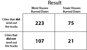
Last April, Treasury Secretary Bessent and DHS Secretary Noem signed a memorandum of understanding allowing ICE to submit names and addresses to the IRS for cross-verification against tax records. ICE submitted 1.28 million names. The IRS returned roughly 47,000 matches. The acting IRS commissioner resigned over the agreement. And Judge Colleen Kollar-Kotelly, reviewing the IRS’s own chief risk officer’s declaration, found that in the vast majority of those 47,000 cases, ICE hadn’t even provided a valid address for the person it was looking for — as required by the Internal Revenue Code. The address fields contained entries like “Failed to Provide,” “Unknown Address,” or simply “NA NA.”³

NA NA.

That’s what ICE typed into the field that was supposed to ensure the government could only access tax records for individuals it had already specifically identified. And the IRS said: close enough.

Now, the obvious story here — the one you’ll get from the news — is about a legal violation and an institutional failure. And that story is correct. But there’s a deeper story, one that requires thinking about what classification systems do to the populations they classify. Because the address field in the §6103 request wasn’t just a data element. It was a constraint — a design specification that determined what kind of system the IRS-ICE pipeline would be. With the address requirement enforced, the system is a targeted lookup: you ask about a specific person you’ve already identified, and the IRS confirms or denies. With the address requirement collapsed — with “NA NA” treated as a valid input — the system becomes a dragnet. Same code, same database, same agencies. But a fundamentally different machine, operating under fundamentally different logic, with fundamentally different consequences for the people inside it.

I want to talk about those consequences. Specifically, I want to talk about what happens to the population being classified when the classifier changes.

---

Filing Taxes as a Strategic Choice

Here’s the setup. If you’ve read the work Maggie Penn and I have been doing on classification algorithms, this will look familiar.⁴

Undocumented immigrants in the United States pay taxes. They do this using Individual Taxpayer Identification Numbers (ITINs), which the IRS issues specifically to people who have tax obligations but aren’t eligible for Social Security numbers. Filing is not optional — the legal obligation exists regardless of immigration status. But the compliance rate — how many people actually file — has historically been sustained by a critical institutional feature: a firewall between tax data and immigration enforcement. Section 6103 of the Internal Revenue Code strictly prohibits the IRS from sharing taxpayer information with other agencies except under narrow, court-supervised conditions.

The firewall is what made tax filing a safe act. Filing carried a compliance benefit — potential refunds, building a record for future status adjustment, staying on the right side of the IRS — and essentially zero enforcement cost. The tax system observed you, but the immigration system couldn’t see what the tax system saw.⁵ To put it in terms we’ll use throughout: the classifier’s expected responsiveness was zero.⁶ When the classifier is null, people make their filing decision based solely on the intrinsic costs and benefits of compliance. Call that sincere behavior.

The MOU blew a hole in that firewall. After the MOU, filing generates a signal — the tax record, including your address — that feeds directly into an enforcement match. Before the breach, the only classifier that mattered was the IRS’s own enforcement system, and that system rewarded filing: if you complied, you reduced your probability of audit, penalty, and all the administrative misery that follows from the IRS noticing you didn’t file. The reward was real, the classifier was responsive to compliance, and the equilibrium worked.

The MOU layered a second classifier on top — the ICE match — and this one runs in the opposite direction. Filing still reduces your IRS enforcement risk, but it now increases your immigration enforcement risk, because filing is what generates the data that feeds the match. For citizens and legal residents, the second classifier is irrelevant — they face no immigration enforcement cost, so the net calculus doesn’t change. For undocumented immigrants, the second classifier dominates. The expected cost of filing went up, and for many people it went up enough to swamp the expected benefit.

The equilibrium compliance rate in the model is

$$\pi_F(\delta, \phi, r) = F(r \cdot \rho(\delta, \phi))$$

where $r$ captures the net stakes of being classified and $\rho$ captures how much the classifier’s decision depends on the individual’s behavior.⁶ When the firewall was intact, the net reward to filing was positive — the IRS classifier rewarded compliance, and the immigration system couldn’t see you. When the firewall broke, the net reward dropped, in some cases below zero, and the filing rate dropped with it. Not because the legal obligation changed. Not because the refund got smaller. Because the classifier changed, and people responded.

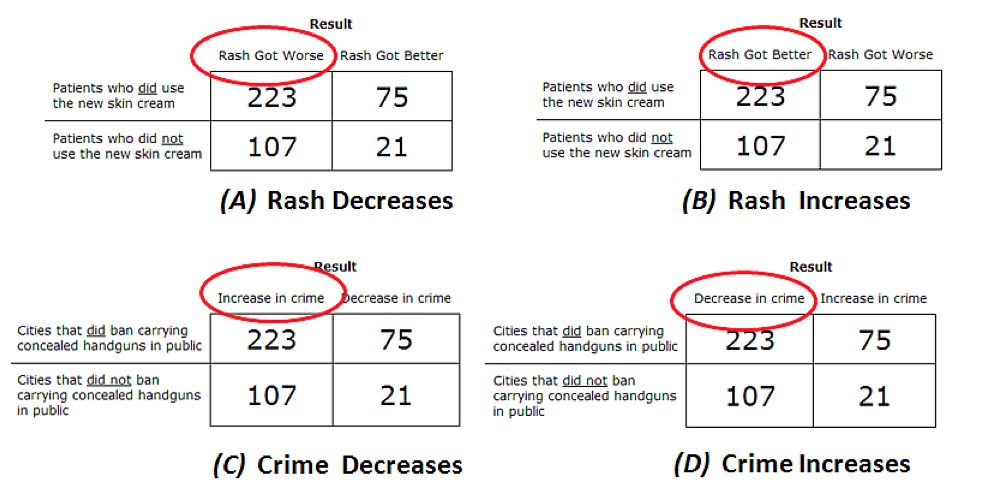
This is a point that’s worth pausing on, because it’s general and it’s important: classification systems do not passively observe the world. They reshape it. A credit-scoring algorithm changes how people use credit. An auditing algorithm changes how people report income. A policing algorithm changes where people walk. The instrument and the thing being measured are not independent of each other, and any analysis that treats them as independent will be wrong in a specific, predictable direction: it will overestimate the accuracy of the system and underestimate its behavioral effects.

Think of two cities, each with a system for issuing speeding tickets. One city’s algorithm is designed to ticket speeders — it cares about accuracy. The other city’s algorithm is designed to generate revenue — it tickets indiscriminately. Drivers in the accuracy-motivated city slow down, because compliance is rewarded. Drivers in the revenue-motivated city don’t bother, because ticketing has nothing to do with their behavior. Same roads, same drivers, same speed limits. Different classifiers, different equilibria. The classifier doesn’t just measure the city — it makes the city.⁷

---

The Death Spiral

This is where it gets interesting. And by “interesting” I mean “bad.”

The people most likely to be correctly identified by the IRS-ICE match are those with stable addresses who file consistently and accurately. These are, almost by definition, the most compliant members of the undocumented population — the ones who’ve been following the rules, building a paper trail, doing exactly what the system told them to do. They’re also the ones with the most to lose from enforcement, because they’ve given the system the most data about themselves.

These are the first people who stop filing.

Judge Talwani flagged this directly. Community organizations that provide tax assistance to immigrants can’t advise their members to stop filing — that would be encouraging illegal behavior. But they also can’t encourage filing, because filing now triggers enforcement risk. The organizations reported decreased revenue and participation. The chilling effect isn’t hypothetical. It’s in the court record.

Now here’s the feedback loop. When the most identifiable filers exit the system, the quality of the remaining data degrades. The match rate goes down. The false positive rate — the probability that a match incorrectly targets a citizen or legal resident — goes up, both because the denominator of correctly matched records shrinks and because ICE is submitting garbage inputs (“NA NA”) that the IRS is accepting anyway. The classifier gets worse at its stated objective precisely because it’s operating.

The system doesn’t just get unfair. It gets worse at its own stated purpose — identifying specific individuals — because the individuals it could most easily identify are exactly the ones who stop showing up.

This is a general property of classification systems with endogenous behavior, and it’s one I think about a lot. When the population being classified can respond to the classifier, the classifier doesn’t observe a fixed distribution. It selects the distribution that’s willing to be observed. And that selection runs in exactly the wrong direction if your goal is accurate identification: the easy cases exit, the hard cases remain, and accuracy deteriorates as a function of the classifier’s own operation. The system eats its own inputs.⁸

---

What the Designer Wants Matters

One of the results Maggie and I are most insistent about is that the objectives of the entity doing the classifying shape the equilibrium in ways that aren’t obvious from the classifier’s structure alone. Two cities with identical data, identical populations, and identical infrastructure but different objectives will design different classifiers, induce different behavior, and produce different social outcomes. The objectives live inside the algorithm, not alongside it.

So: what is DHS trying to do?

The official framing is accuracy-aligned. DHS says the goal is to “identify who is in our country.” That sounds like accuracy maximization: correctly match individuals to their immigration status.

But the implementation tells a different story. An accuracy-maximizing designer needs good inputs — the whole point of the §6103 requirement that ICE provide a valid address is to ensure the system operates on pre-identified individuals, which is a precondition for accurate matching. ICE submitted “NA NA.” They submitted jail addresses without street locations. They submitted 1.28 million names and got 47,000 matches, meaning a 96.3% non-match rate before you even get to the question of whether the matches were accurate.

This doesn’t look like accuracy maximization. It looks like a fishing expedition — a bulk data pull designed to maximize the reach of the enforcement system rather than the precision of individual identifications. In the language of the paper, it looks more like compliance maximization (or its dark inverse: maximizing the chilling effect on a target population) or outright predatory objectives — a system that benefits from inducing non-compliance, because non-compliance makes the targets more vulnerable, not less.⁹

And the distinction between objectives matters formally, because the two produce different classifiers with different welfare properties. An accuracy-maximizing classifier, we show, will push some groups toward compliance and others away — exacerbating behavioral differences between groups even when the data quality is identical across groups. A compliance-maximizing classifier, by contrast, always satisfies what we call aligned incentives: it pushes all groups in the same behavioral direction.

Here, the groups aren’t abstract. They’re citizens, legal residents, and undocumented immigrants, all of whom file taxes, all of whom had their data swept into the same match, and all of whom face different enforcement costs from being identified. The classifier doesn’t distinguish between them at the input stage — it just matches names and addresses. But the behavioral response to the classifier differs radically across groups, because the stakes of being classified differ radically. Citizens face essentially zero enforcement cost from a match. Undocumented immigrants face deportation. The same classifier, applied to the same data, produces wildly different equilibrium behavior in different populations.

That’s not a bug in the implementation. That’s a structural property of classification systems with heterogeneous stakes. And it’s a property that accuracy maximization makes worse, not better.

---

The Commitment Problem

There’s one more piece of the model that’s eerily relevant. We distinguish between designers who can commit to a classification algorithm and designers who are subject to audit — who must classify consistently with Bayes’s rule and their stated objectives. The commitment case is more powerful: a designer who can commit can deliberately misclassify some individuals to manipulate aggregate behavior. The no-commitment case, which we interpret as the effect of auditing or judicial review, strips away this power.

Judge Kollar-Kotelly’s ruling is an audit. She looked at what the IRS actually did — accepted “NA NA” as a valid address, disclosed 42,695 records in violation of the statutory requirement — and said: this doesn’t satisfy the constraints. Judge Talwani’s injunction goes further, blocking enforcement use of the data entirely.

These rulings function exactly as the no-commitment constraint does in the model. They force the classifier to satisfy sequential rationality — to justify each classification decision on its own terms, rather than as part of a bulk strategy to influence population behavior. And the paper tells us what happens when you impose that constraint: the resulting equilibrium satisfies aligned incentives. The designer can no longer push different groups in different behavioral directions.

That’s the fairness argument for judicial review of classification systems, stated formally. It’s not that judges know better than agencies how to design algorithms. It’s that the constraint of having to justify individual decisions prevents the designer from using the algorithm to strategically manipulate aggregate behavior. The cost is accuracy — the no-commitment equilibrium is always weakly less accurate than what the designer could achieve with commitment power. But the benefit is behavioral neutrality across groups, which is a fairness property that accuracy maximization cannot guarantee.¹⁰

---

Where This Goes

The D.C. Circuit will rule on the Kollar-Kotelly injunction. If they uphold it, the no-commitment constraint holds and the data-sharing agreement is dead in its current form. If they reverse — and the Edwards panel’s reasoning from two days ago suggests this is possible — the commitment case reasserts itself, and the behavioral distortions I’ve described become the operating equilibrium.

Meanwhile, the chilling effect is already in motion. People have already stopped filing. Community organizations have already seen decreased participation. The equilibrium is shifting in real time, and it won’t shift back quickly even if the courts ultimately block the agreement, because trust in the firewall is not a switch you can flip. It’s a belief about institutional behavior, and beliefs update slowly after violations — especially violations that occurred 42,695 times.

The tax system was designed as a compliance mechanism: file your returns, pay what you owe, and we won’t use your data against you. That design was a choice. The firewall was a choice. The address requirement in §6103 was a choice. Every one of those choices encoded a judgment about what the system should be for — not just what it should measure, but what kind of behavior it should sustain. The MOU didn’t just breach a legal firewall. It changed the classifier, which changed the equilibrium, which is changing the population, which will change the data, which will change what the classifier can do. The whole thing is a loop, and it’s spinning in exactly the direction the model predicts.

I said I’d be back when something in the news was so perfectly illuminated by the theory that I couldn’t not write about it. This is that. There will be more.¹¹

With that, I leave you with this.

---

^{1. 72.9%, for those keeping score. ↩}

^{2. The phrase is from Li and Yorke’s 1975 paper “Period Three Implies Chaos,” which proved that a continuous map with a periodic point of period 3 has periodic points of every period — plus an uncountable mess of aperiodic orbits. But the tagline does triple duty: Arrow’s theorem, the Gibbard-Satterthwaite theorem, and the McKelvey-Schofield chaos theorem all say that with three or more alternatives, the relationship between individual preferences and collective outcomes becomes fundamentally unstable. Norman Schofield, who proved the general form of the chaos result with Richard McKelvey, was a mentor and colleague to both Maggie Penn and me at Washington University. It was Norman, in a bar in Barcelona, who suggested that Maggie and I write our first book, Social Choice and Legitimacy: The Possibilities of Impossibility, which we dedicated in part to McKelvey. He died in 2018, and he is one of the people I miss when I write here. Three implies chaos. It’s not a bug. It is the central fact of democratic life. ↩}

^{3. The legal landscape is, to use a technical term, a mess. Kollar-Kotelly’s injunction from November is still in effect but under appeal in the D.C. Circuit. Judge Talwani in Massachusetts issued a separate injunction in early February blocking enforcement use of the data. And two days ago, a D.C. Circuit panel declined to enjoin the agreement, reasoning that “last known address” isn’t protected return information under §6103. So you have district courts saying it’s illegal and an appellate panel suggesting it might not be. Three courts, three bins for the same data. If that doesn’t sound like a social choice problem to you, you haven’t been reading this blog long enough. ↩}

^{4. Penn and Patty, “Classification Algorithms and Social Outcomes,” American Journal of Political Science (forthcoming). The formal model and all the results I’m drawing on here are in that paper. What follows is a blog-post-grade application of the framework, not a formal extension of it. But the shoe fits disturbingly well. ↩}

^{5. The firewall wasn’t just a policy preference — it was constitutional load-bearing infrastructure. The government’s power to tax illegal income was established in United States v. Sullivan (1927) and famously applied to convict Al Capone in 1931. But requiring people to report illegal income creates an obvious Fifth Amendment problem: filing becomes compelled self-incrimination. Section 6103 resolved the tension by ensuring tax data stayed behind the wall. With the firewall intact, you could — in principle — write “narco drug lord” in the occupation field of a 1040 and nothing would happen, because the IRS couldn’t share it. The MOU reopened that wound. If filing now feeds ICE, then filing is self-incrimination for undocumented immigrants, and the constitutional bargain that made the whole system work since Sullivan is back in play. Whether anyone is litigating this yet is a question I leave open, but the logical structure is Gödelian: the system simultaneously compels disclosure and punishes the act of disclosing. ↩}

^{6. In the model, expected responsiveness is $\rho(\delta, \phi) = (\delta_1 + \delta_0 – 1)(2\phi – 1)$, where $\delta_1$ and $\delta_0$ are the probabilities that the classifier’s decision matches the signal for compliers and non-compliers respectively, and $\phi$ is signal accuracy. A null classifier has $\rho = 0$: the probability of being targeted is the same regardless of whether you file. The §6103 firewall enforced nullity by severing the link between the signal (tax record) and the decision (enforcement action). ↩}

^{7. This example is from the paper, but it’s the kind of thing that should be folklore by now. It isn’t, largely because the computer science literature on algorithmic fairness has mostly treated the classified population as fixed. That’s starting to change — see Perdomo et al. (2020) on performative prediction and Hardt et al. (2016) on equality of opportunity — but the political science framing, where the designer has objectives and the population has strategic responses, is still underdeveloped. Maggie and I are trying to fix that. ↩}

^{8. There’s also a revenue dimension that shouldn’t be ignored. The IRS estimates that undocumented immigrants pay billions in federal taxes annually. If the filing rate drops — which it will, and which the court record suggests it already is — that’s tax revenue the government doesn’t collect. The classifier was supposed to serve immigration enforcement, but its equilibrium effect includes degrading the tax base. Whether anyone in the administration has done this calculation is an exercise I leave to the reader. ↩}

^{9. Predatory preferences in the model are characterized by a designer whose most-preferred outcome is to not reward an individual who didn’t comply. Think predatory lending: the lender benefits most when the borrower defaults, because the default triggers fees, repossession, or refinancing at worse terms. A designer with predatory preferences over immigration enforcement would want undocumented immigrants to stop filing taxes, because non-filers are more legally precarious, have weaker paper trails, and are easier to deport. Whether this is what DHS actually wants is a question I can’t answer from the model. But the model can tell you what the observable signatures of predatory preferences look like, and “submit NA NA as an address for 1.28 million people” is consistent with the signature. ↩}

^{10. Whether you think that tradeoff is worth it depends on what you think “fairness” means in this context, and reasonable people disagree. But the point is that it is a tradeoff, with formal properties that can be characterized — not a vague gesture at competing values. I have more to say about this, and about how it connects to a set of problems that go well beyond tax data. But that will have to wait for another post. Or, you know, the book. ↩}

^{11. Next up: the Supreme Court just handed us a game-theoretic goldmine, and three implies chaos. Stay tuned. ↩}