Mind The Gap: The Wages of Aggregation, Evaluation, and Conflict

For whatever reason, I’m on a “data is complicated kick.”

So, this story is one of many today discussing the gender gap in wages in ‘Merica. In a nutshell, President Obama pointed out “that women make, on average, only 77 cents for every dollar that a man earns.”  Critics (most notably the American Enterprise Institute) immediately pointed out that “the median salary for female employees is $65,000 — nearly $9,000 less than the median for men.”

There are LOTS of angles on this thorny issue.  I want to raise the specter of social choice theory as a mechanism by which we can understand why this debate goes around and around.[1] The basic idea is that aggregation of data involves simplification, which involves assumptions.  Because there are various assumptions one can make (properly driven by the goal of one’s aggregation), one can aggregate the same data and reach different conclusions/prescriptions.

To keep it really simple, consider the following toy example.  Suppose that a manager currently has one employee, who happens to be a man, who makes $65,000/year, and the manager has to fill three positions, A, B, and C.  Furthermore, suppose that the manager has a unique pair of equally qualified male and female applicants for each of these three positions.  Finally, suppose that position A is paid $70,000/year, position B is paid $60,000/year, and position C is paid $45,000/year.

Now consider two criteria:

(1) eliminate/minimize the gender gap in terms of average wages,[2] and
(2) minimize the difference between proportions of male and female employees.

How would the manager most faithfully fulfill criteria (1)?  Well, if you hire the woman for position B and the two men for positions A and C, then the average wage of women (i.e., the woman’s wage) is $60K, and the average of the three men’s (the existing employee and the two new employees) wages is $60,000.  This is clearly the minimum achievable.[3]

How about criteria (2)?  Well, obviously, given that one man is already employed, the manager should hire two women.  If the manager satisfies criteria (2) with an eye toward criteria (1), then the manager will hire a man for position B and women for positions A and C.

Note that the two criteria, each of which has been and will be used as benchmarks for equality in the workplace (and elsewhere), suggest exactly and inextricably opposed prescriptions for the manager.

In other words, the manager is between a rock and a hard place: if the manager faithfully pursues one of the criteria, the manager will inherently be subject to criticism/attack based on the other.

Note that this is not “chaos”: the manager, if faithful, must hire no more than 2 of either gender: hiring three men or three women is incompatible with either of these criteria.[4] But the fact remains—and this is a “theory meets data” point—one can easily (so easily, in fact, that one might not even realize it) impose an impossible goal on an agent if one uses what I’ll call “data reduction techniques/criteria” to evaluate the agent’s performance.

In other words: real world politics is inherently multidimensional.  When we ask for simple orderings of multidimensional phenomena (however defined, and of whatever phenomena), we are in the realm of Arrow’s Impossibility Theorem.

_________

[1] This argument is made in a more general way in my forthcoming book with Maggie Penn, available soon (really!) here: Social Choice and Legitimacy: The Possibilities of Impossibility.

[2] Here, by “average,” I mean arithmetic mean.  Because this example is so small, there is no real difference between mean, median, and mode in terms of how one measures the gender gap.  If these differ in practice, then the problem highlighted here is merely (and sometimes boldly) exacerbated.

[3] To be clear, I am setting aside the issue of “how much does a gender make if none of that gender is employed?” While technically undefined, I think $0 is the most common sense answer, and I’ll leave it at that.  

[4] Of course, as Maggie Penn and I discuss in our aforementioned book, there are many criteria.  Our argument, and that presented in this post, is actually strengthened by arbitrarily delimiting the scope of admissible criteria.

It’s Better To Fight When You Can Win, Or At Least Look Like You Did

In this post, Larry Bartels provocatively claims that Rich People Rule! In a nutshell, Bartels argues (correctly) that more and more political scientists are producing multiple and smart independent analyses of the determinants of public policy, one of which, by Kalla and Broockman, I have already opined on (“Donation Discrimination Denotes Deliverance of Democracy“).

Bartel’s motivation for bringing this up is essentially this quote from this forthcoming article by Martin Gilens & Benjamin Page:

economic elites and organized groups representing business interests have substantial independent impacts on U.S. government policy, while mass-based interest groups and average citizens have little or no independent influence.

The Gilens and Page is an interesting read, if only because the data on which it is based is very impressive.

Unfortunately, the theory behind the work is not nearly as strong.  In particular, the study is based on comparing observed position-taking by interest groups with (solicited) individual feedback on various surveys.[1]  So what?  Well, there is at least one potential problem, containing two sub-points, the combination of which I’ll call the Pick Your Battles Hypothesis.

Pick your battles.  Interest groups do not randomly announce positions on public issues.  Rather, any interest group of political interest presumably attempts to influence public policy through strategic choices of not only what to say, but when to bother saying anything at all.  While the mass public opinion data was presumably gathered by pollsters in ways to at least somewhat minimize individuals’ costs of providing their opinions, the interest groups had to pay the direct and indirect costs of getting their message(s) out. There’s two sub-points here, one more theoretical interesting than the other and the other presumably more empirically relevant.

Sub-point 1: Pick a winner. The theoretically interesting sub-point is that an organized “interest group” is/are the agents of donors and supporters.  To the degree that donations and support are conditioned on the perceived effectiveness of the interest group, (the leaders/decision-makers of) an interest group will—ala standard principal-agent theory—have a greater incentive to pay the costs of taking a public position when they perceive that they are likely to “win.”  If there is such a selection effect at work, then the measured correlation between policy and interest groups’ positions will be overestimated.

Sub-point 2: Only Fight The Fights That Can Be Won. The more empirically relevant sub-point is that, even if one thinks that interest groups don’t fear being on the losing side of a public debate, the simple and cold reality of instrumental rationality is that, if making an announcement is costly, any interest group should make an announcement only when the announcement can actually affect something.  Moving quickly here, this suggests that interest groups should be taking positions when they believe decision-makers might be persuaded.  To the degree that these decision-makers are presumably at least somewhat responsive to public opinion (however measured), instrumentally rational (and probably asymmetrically informed) interest groups will be more likely to make announcements that run against relative strong public opinion than to join the chorus.[2]  If this is happening, the question of whether interest groups have too much influence depends on whether you think they have better or worse information and on the types of policies that their views are influential on.

Conclusion. As political scientists know, observational data is tricky.  This is particularly true when it is the result of costly individual effort in pursuit of policy (and other) goals.  I really like Gilens and Page’s paper—the realistic point of scholarly inquiry is not to be right, it’s to get ever closer to being right, and this is even more true with directly policy-relevant work.  I just think that great data should be combined with at least a modicum of (micro-founded, individualistic) theoretical argument.  Without that, we might think umbrellas cause rain, hiring a lawyer causes you to go to jail, or chemotherapy causes death from cancer.  In other words, the analyst has simultaneously more data and less information than those he or she studies.

_______________

[1] Gilens and Page also compare responsiveness to mass opinions of economic elites (i.e., those in the 90th percentile in income) versus those of the median earner.  While I have some issues with this comparison (for example, I imagine getting a representative sample of the 90th income percentile is a bit different than getting one of the median income earner and, as Gilens and Page acknowledge, the information held by and incentives of the rich are plausibly very different from those of median earners), I will focus on the interest group component of the analysis in this post.

[2]  That this is not just hypothetical crazy talk is indicated by the relatively strong negative correlation (-.10***) between the positions of business interest groups and the average citizen’s preferences.


Donation Discrimination Denotes Deliverance of Democracy

A recent paper by Joshua Kalla & David Broockman has attracted some attention (for example, in this Washington Post storyMonkey Cage post, and this excellent, reflective post on Mischiefs of Faction by Jennifer Victor).  In a nutshell, the paper reports the results of a well-designed field experiment that provides evidence that donations to a Member of Congress “open doors” in the sense that being a donor promotes access to more high ranking officials in the Member’s staff, including possibly the Member of Congress himself or herself.

I am not going to critique the study. Jennifer does that well in several ways.  Unrelatedly, I am also not going to doubt (or cast doubt upon) the results.  Rather, doing what I do, I am going to make a quick point about the question at hand.

We have a situation in which a (quasi-)monopolist (the Member) has a “good” to sell (access/face time).  Simply put, let’s suppose this good is valuable to some people and, similarly, that donations are valuable to the Member.  Then, it follows from a classic corner of social science known as price discrimination that the Member (in self-interested terms) should privilege those who are willing to pay for it.  That is, those who want access most will be willing to pay more than those want access less, and an efficient means to allocate the scarce/costly resource of access is to give to those who are most willing to pay.  Is this normatively disturbing?  Hell, yes.  Is it troubling even in everyman’s language?  Oh, for sure.  Is it inevitable?  Well, yes, that too.

Here’s another, more methods-meets-theory take on it.  Suppose that a Member imposed a policy where donations did not offer an advantage in obtaining access.   Now, think about your position as a constituent/citizen seeking access.

What would you do?

Let’s suppose that you like money. We’ve already supposed you seek access.  Now, finally, put those two together in the face of the hypothetical Member who does not reward donations with preferential access. … You should be very happy as you realize that you can have your cake and eat it, too, as you keep your money and waltz into the Member’s office, swilling sherry and talking Grand Strategy into the wee hours.

The summary of this hypothetical is this: if you believe that is plausible (1) that members don’t reward donations with preferential access and (2) that potential donors like money, then the predicted level of donations to any members is zero.[1]

We know that people give money to campaigns.  We also know or at least strongly believe that people expect something for their money.  Putting these together, I will simply say that the conjunction of these makes me feel better, not worse, about our democratic system.

Paraphrasing at least an apocryphal version of Churchill, democracy is better than every system we’ve ever tried, but it’s still only capable of delivering second-best…at best.  The Kalla & Broockman results, as clean as a whistle, further confirm my belief in this.


_________

[1] This is a blog post, and I’ve been away for a while for many reasons, including that these take me a lot of time.  Accordingly, I’ll simply note that other motivations for giving (e.g., financing reelection campaigns in a purely instrumental fashion) can be accomplished by other routes in the Federal campaign finance system (party committees, other PACs, etc., and unless you are really focused on a given Member’s reelection (but why, except for access?), these routes have transaction costs/flexibility advantages over direct giving to a single Member’s campaign).

Ceiling the Deal: Quid Pro Keystone

The debt ceiling drama is inexorably drawing to its next installment, and the question remains: when and, more importantly, how will a deal get done?  To keep matters simple, President Obama and Congressional Democrats have stood by the long-standing pledge to not negotiate on the debt ceiling, but some Congressional Republicans have been pushing for concessions in return for a debt ceiling increase—in particular, approval of the Keystone XL pipeline.

The State Department released its final report on the environmental impact of the proposed Keystone XL pipeline (fact sheet here) last week.  In a nutshell, the report is a “win” for pipeline supporters.  The idea of a “Keystone approval in return for debt ceiling increase” deal is not new, of course.  What I want to discuss briefly is the procedural details of the deal and their strategic (electoral) implications.

A key question in this game is whether Congress explicitly attaches Keystone XL approval to the debt ceiling increase or not.  Congress could pass a combined bill, or perhaps an implicit deal will be struck: President Obama approves Keystone XL and Congressional Republicans approve a “clean” debt ceiling increase, without (too loudly) claiming a quid pro quo.

I have reason to suspect that President Obama is trying to set up exactly such a deal: he said in June that the criterion for approving the pipeline is that is “not significantly exacerbate the problem of carbon pollution.”  The State Department report provides an argument that it won’t.  Furthermore, President Obama said that “the net effects of the pipeline’s impact on our climate will be absolutely critical to determining whether this project is allowed to go forward.

However, White House press secretary Jay Carney said today that Obama’s decision on the pipeline would be free from “ideological or political influence.” And the current spin regarding Secretary of State Kerry is that (1) Obama has asked him for a recommendation on the project and (2) that Kerry may be conflicted regarding his principles and partisan motivations.

The strategic question here for my purposes today is

Does Obama value “not bargaining” over the debt ceiling—a signaling of resolve, etc. that I have touched upon in various other posts (such as here)—more than the potential gain from allowing moderate Democratic Senators to vote for a bill (perhaps with a debt ceiling increase too) mandating approval of the project? [1] [2]

With respect to the first point, I think all three sides (Democrats, Republicans, and Canadians) are playing a bit of a game of chicken: nobody wants to be seen as “giving in” if they don’t have to.  I won’t work this through in detail, but the basics of “chicken” as pretty simple: each player would prefer to look tough (not give in) and have one or both of the others give in.[3]  At the same time, each player would prefer to give in if they knew that neither of the others were going to give in.  The best case scenario in this situation, it seems, is the “win-win” scenario of (1) Obama looking “presidential” and “job-creating” by solemnly approving the Keystone project at the same time as (2) Congress passing a “dirty” debt ceiling increase that mandates approval of the pipeline.

The devil, of course, is in the details: the timing has to be managed appropriately so that neither side is “clearly” trying to save face.  I think this can be accomplished by having the Senate vote for a Keystone approval and clean debt ceiling increase separately, then have the House vote under a special rule to approve both and send them to the President, during which time the President would unilaterally approve the pipeline, so that he could explain that he was essentially signing a clean debt ceiling increase.

Will it work out this way?  Oh, I’m sure it will be different.  But with the benefit of being “up close” in temporal terms, I would be somewhat surprised if we don’t see action on both the debt ceiling and the Keystone project in the next week.

With that, I leave you with this.

_____________

[1] In 2012, a majority of the Senate voted in favor of such an approval, though it failed to get the 60 votes required to move forward.

[2] I thought about discussing why Obama might want a visible and positive Kerry recommendation, versus why he might want a negative and visible one.  The basics of one such argument are provided by my colleague Randy Calvert’s seminal article from 1985, entitled “The Value of Biased Information.”  I’ll come back to this argument at another time, I’m sure.  (And, to be honest, I have already stood on Randy’s shoulders elsewhere.)

[3] Usually, “Chicken” is described as a two-player game.  With more than 2 players, it becomes clear that Chicken is really just “private provision of a public good,” or the “who takes the trash out game.”  This is not the same as the Who Let The Dogs Out? game, which has no pure strategy equilibria (Baha Men (2000)).

Poor Work Counting the Working Poor

This Op-Ed in Forbes, “Almost Everything You Have Been Told About The Minimum Wage Is False,” by Jeffrey Dorfman, argues that increasing the federal minimum wage (1) would not affect as many people as you might think and (2) would not help the working poor as much as (say) teenagers.

The first half of Dorfman’s Op-Ed is misleading in important and ironic ways.[1]  I will detail three significant logical failures in it, and then provide a more transparent accounting of how many people’s wages would be directly increased by an increase of the federal minimum wage to $10.10/hr.

Three Failures. First, Dorfman either misunderstands or misrepresents the difference between necessary and sufficient conditions when he writes:

First, people should acknowledge that this rather heated policy discussion is over a very small group of people. According to the Bureau of Labor Statistics there are about 3.6 million workers at or below the minimum wage (you can be below legally under certain conditions). 

Dorfman should acknowledge that raising the federal minimum wage would affect not only those who earn a wage less than or equal to the current minimum wage.  The data that Dorfman is discussing excludes anybody who receives $7.26/hr or more.  Thus, Dorfman should acknowledge that the “small” group of 3.6 million people he is considering compose the relevant basis of discussion if we are considering a one cent increase in the federal minimum wage.[2]

Second, Dorfman starts comparing apples and oranges, writing

Within that tiny group, most of these workers are not poor and are not trying to support a family on only their earnings. In fact, according to a recent study, 63 percent of workers who earn less than $9.50 per hour (well over the minimum wage of $7.25) are the second or third earner in their family and 43 percent of these workers live in households that earn over $50,000 per year.

This is apples to oranges because the data in the (linked) study is from 2003-2007, before the Great Recession, but the BLS data is from 2012. Furthermore, Dorfman doesn’t take the time to actually report what the study does say (on page 593):

Of those who will gain, 63.2% are second or third earners living in households with incomes twice the poverty line, and 42.3% live in households with incomes three times the poverty line, well above $50,233, the income of the median household in 2007.

Let’s think about this for a second: ~20% of those who made less than $9.50/hr in 2007 lived in a household with an annual income (it turns out) of somewhere between $41,300 and $61,950.  I mean, seriously, helping this kind of household—you know, hard-working and distinctly middle class—that would be a ridiculous outcome.

In addition, I’m going to be quick about Dorfman’s faulty (and, I think, disingenuous) logic in his implication that people poorly paid job “… are not trying to support a family on only their earnings” just because others in the household are working, too.

Namely, if you are the second or third earner in a family, that does not imply that you don’t need the money.  In fact, I am going to blatantly assert that it’s probably the case that the number of “voluntarily non-working” 16+ year-olds in an American household is positively correlated with the household’s income.  After all, many people work a job for, you know, the money.  But, of course, some people might take near-minimum-wage jobs just to keep themselves busy.

Next, Dorfman starts making descriptive statements out of the blue:

...Thus, minimum wage earners are not a uniformly poor and struggling group; many are teenagers from middle class families and many more are sharing the burden of providing for their families, not carrying the load all by themselves.

The closest thing Dorfman putatively offers as evidence for the conclusion that these are teenagers (there is no evidence from what kind of families these teenagers come in the BLS data) is the BLS data, which again is constrained only to those earning no more than the minimum wage of $7.25/hr.

Finally, Dorfman says

This group of workers is also shrinking. In 1980, 15 percent of hourly workers earned the minimum wage. Today that share is down to only 4.7 percent. Further, almost two-thirds of today’s minimum wage workers are in the service industry and nearly half work in food service. 

But again, the point is that raising the minimum wage to (say) $10.10/hr, as President Obama has called for, would help more than only those who earn the minimum wage.

I’m not just going to point out Dorfman’s mistakes.  I have done a little digging (it took me about 15 minutes, to be clear, to get real numbers), and I’ll give a better estimate of how big that “very small group of people” really is.[3]

The Occupational Employment Statistics Query System, provided by the U.S. Bureau of Labor Statistics, provides a different picture of how many people would be impacted by a change in the federal minimum wage to $10.10/hr.

The most recent data, from May 2012, is displayed at the end of this post.  The points I’d like to quickly point out are as follows:

  • In Food Preparation and Serving Related Occupations, 50% of 11,546,880 workers receive less than $9.10/hr, and 75% receive less than $11.11/hr.  Thus, somewhere around 62.5% of these workers, or about 5.75 million people would receive a higher wage.
  • In Sales and Related Occupations, 25% of 13,835,090 workers receive less than $9.12/hr, and 50% receive less than $12.08/hr.  So, conservatively, about 3.5 million people would receive a higher wage.
  • In Transportation and Material Moving Occupations, 25% of 8,771,690 workers receive less than $10.06/hr.  Thus, over 2.1 million people would receive a higher wage.
  • In Healthcare Support Occupations, 25% of 3,915,460 workers receive less than $10.03/hr.  That’s nearly a million people who would receive a higher wage.
  • Overall, 10% of all workers (across all industries) receive an hourly wage lower than $8.70/hr, and 25% of all workers receive an hourly wage lower than $10.81/hr.  A rough estimate, then, is that at least one out of every six workers would receive a higher hourly wage if the federal minimum wage were raised to $10.10/hr. To put that in absolute terms:

Over 21,500,000 Americans would receive a higher wage.

…or, about 6 times as many as Dorfman implied.


With that, I leave you with this.

___________________

[1] I will not address the second part of Dorfman’s piece about productivity shifts in the food service industry, and the “ironic” aspect of the mistakes in the piece is the conclusion of the first paragraph, where Dorfman informs the reader that “much of what you hear about the minimum wage is completely untrue.”

[2] I am setting aside the question of how many people who currently earn less than minimum wage would be affected by an increase in the level of the wage.  This is a complicated matter for a variety of reasons.

[3] I, like Dorfman, will leave aside the question of overall impact of a minimum wage hike on employment.  I am not advocating for or against a minimum wage hike—rather, I am advocating against those who argue that very few workers make very low wages.

___________________


BLS Data:


Occupation (SOC code) Employment(1) Hourly mean wage Hourly 10th percentile wage Hourly 25th percentile wage Hourly median wage Hourly 75th percentile wage Hourly 90th percentile wage Annual 10th percentile wage(2) Annual 25th percentile wage(2) Annual median wage(2)
All Occupations(000000) 130287700 22.01 8.70 10.81 16.71 27.02 41.74 18090 22480 34750
Management Occupations(110000) 6390430 52.20 22.12 31.56 45.15 65.20 (5)- 46000 65650 93910
Business and Financial Operations Occupations(130000) 6419370 33.44 16.88 22.28 30.05 40.61 53.50 35110 46340 62500
Computer and Mathematical Occupations(150000) 3578220 38.55 19.39 26.55 36.67 48.40 60.55 40330 55220 76270
Architecture and Engineering Occupations(170000) 2356530 37.98 19.45 26.16 35.35 46.81 59.52 40450 54420 73540
Life, Physical, and Social Science Occupations(190000) 1104100 32.87 15.06 20.35 28.89 41.18 55.38 31320 42330 60100
Community and Social Service Occupations(210000) 1882080 21.27 11.21 14.57 19.42 26.52 34.36 23310 30310 40400
Legal Occupations(230000) 1023020 47.39 16.80 23.15 36.19 62.57 (5)- 34940 48150 75270
Education, Training, and Library Occupations(250000) 8374910 24.62 9.94 14.66 22.13 30.85 41.54 20670 30490 46020
Arts, Design, Entertainment, Sports, and Media Occupations(270000) 1750130 26.20 9.42 13.76 21.12 32.16 46.12 19600 28630 43930
Healthcare Practitioners and Technical Occupations(290000) 7649930 35.35 14.84 20.56 28.94 40.69 61.54 30870 42760 60200
Healthcare Support Occupations(310000) 3915460 13.36 8.62 10.03 12.28 15.64 19.51 17920 20850 25550
Protective Service Occupations(330000) 3207790 20.70 9.09 11.71 17.60 26.89 37.35 18910 24370 36620
Food Preparation and Serving Related Occupations(350000) 11546880 10.28 7.84 8.38 9.10 11.11 14.60 16310 17430 18930
Building and Grounds Cleaning and Maintenance Occupations(370000) 4246260 12.34 8.12 8.95 10.91 14.44 18.93 16890 18630 22690
Personal Care and Service Occupations(390000) 3810750 11.80 7.96 8.66 10.02 13.10 18.21 16560 18010 20840
Sales and Related Occupations(410000) 13835090 18.26 8.25 9.12 12.08 20.88 35.60 17170 18970 25120
Office and Administrative Support Occupations(430000) 21355350 16.54 9.17 11.51 15.15 20.18 26.13 19070 23940 31510
Farming, Fishing, and Forestry Occupations(450000) 427670 11.65 8.23 8.65 9.31 12.97 18.64 17130 18000 19370
Construction and Extraction Occupations(470000) 4978290 21.61 11.15 14.37 19.29 27.19 35.61 23190 29900 40120
Installation, Maintenance, and Repair Occupations(490000) 5069590 21.09 10.92 14.56 19.72 26.63 33.69 22720 30290 41020
Production Occupations(510000) 8594170 16.59 9.02 11.05 14.87 20.26 27.11 18760 22990 30920
Transportation and Material Moving Occupations(530000) 8771690 16.15 8.56 10.06 13.92 19.41 26.83 17800 20930 28960
Footnotes:
(1) Estimates for detailed occupations do not sum to the totals because the totals include occupations not shown separately. Estimates do not include self-employed workers.
(2) Annual wages have been calculated by multiplying the hourly mean wage by 2,080 hours; where an hourly mean wage is not published, the annual wage has been directly calculated from the reported survey data.
(5) This wage is equal to or greater than $90.00 per hour or $187,199 per year.
SOC code: Standard Occupational Classification code — see http://www.bls.gov/soc/home.htm

Data extracted on January 30, 2014


Inequality: Smaller GINIs Can Fit in Smaller Bottles

I have been thinking a lot lately about this very interesting post by Kristina Lerman.  The post is excellent: succinct and well-written, data-centric, and relevant beyond the data’s idiosyncratic qualities.  In a nutshell, Lerman’s central question is whether the rate of information production is outstripping the rate at which we (choose to or can) consume and digest it.

Of course, information overload is clearly an important problem for scholars and practitioners alike (and, accordingly, not one with any obvious and easy answer). But upon reflection, I am still wondering whether it is a problem at all.  Given my second-mover advantage, I will cherry-pick one of the arguments in the post.

In a section titled “Rising Inequality,” Lerman uses the Gini coefficient of citations to physics papers as a measure of scholarly inequality.  Since the Gini coefficient has grown over the past 6 decades, Lerman concludes that “a shrinking fraction of papers is getting all the citations.”  This is undoubtedly true once one slightly rewords it as “a shrinking fraction of the papers made available is getting all the citations.”  This is an important qualifier, in my opinion, and the central point of this post.

Any notion of inequality is inherently relative. As I read it, Lerman’s argument is that the increase in information production has potentially caused us to use cues or heuristics to manage the decision of what information we as scholars consume.  Lerman argues that this is bad because the Gini coefficient has increased along with the rate of publication, indicating that the cues and heuristics we are employing is narrowing our attention to a smaller set of articles and creating a “rich get richer” dynamic in terms of citations and scholarly focus.

However, is this conclusion warranted by the data?  I am not so sure: the Gini coefficient, like any measure of inequality, is potentially sensitive in counterintuitive ways to the set of things being compared to one another.

The nature of Gini coefficients. Lerman’s argument that higher Gini coefficients are bad is very sensible if one thinks that the “pie” of citations is fixed in size and/or that the low citation articles are somehow “unjustly” receiving fewer citations.  At least in my opinion, neither of these suppositions is reasonable in this context.  There’s a number of ways to skin this cat, but I think this is the easiest.  Suppose, for the sake of argument, that the number of citations an article will receive is independent of the number of articles uploaded (or, accepted into an APS journal).  Then, suppose that only those articles that will receive m citations are uploaded.  As the costs of uploading/writing/publishing decrease, m would presumably decrease as well.  With this in hand, the key question is:

Holding the latent population of articles fixed, how does the Gini coefficient of the uploaded articles change as m increases?

Note that decreasing m increases the number of articles uploaded.  To me, at least, Lerman’s implicit argument is that decreasing m “should” decrease inequality (i.e., decrease the Gini coefficient).

This isn’t necessarily the case.  I ran a simulation to demonstrate this with a very large set of “pseudo-data.”  Specifically, I generated 100,000 observations from a Pareto(k=1,\alpha
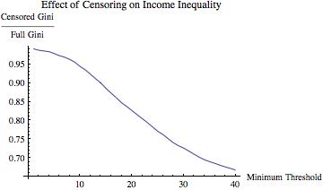
=1.35) distribution.  This pseudo-data yielded a Gini coefficient of \approx 0.59
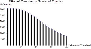
.  Then I truncated the distribution at various values of m\in \{1,2,\ldots,25\} 
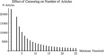
and computed the ratio of the Gini coefficient of the resulting truncated data set and the Gini coefficient of the full data set. If decreasing m “should” decrease inequality, then this ratio should be increasing in m.
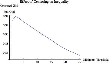
The results are displayed below

CitationGiniRatio CitationSurvivors

The simulated data demonstrate that increasing the selectivity of the upload/publication process can actually decrease inequality among the (changing set of) uploaded/published papers.  In other words, increasing the rate of uploading/publication of articles can increase inequality without reference to information overload or any changes in citation behavior

Out of curiosity, I went out and got some real data. For simplicity, I downloaded the per capita personal incomes of each US county for 2011 (available here).  This data looks like this:

PersonalIncomeHistogram

I then did an analogous analysis, varying the income threshold from $20,500 to $40,000, computing the ratio of the Gini of the truncated data to the Gini of the overall data set at each increment of $500.  The results of this are below.PersonalIncomeGiniRatioPersonalIncomeSurvivors

Again, as one gets more “elite” with respect to the inclusion of a county in terms of income into the calculation of the Gini coefficient, estimated inequality decreases.

Now, it is probably very simple to find examples in which the opposite conclusion holds.  But that’s not the point: I am not arguing that Lerman is wrong.  Rather, I am making a point about inequality measurement in general.  In line with my earlier point about Simpson’s paradox and education policy, comparing relative performance between different sets-even nested ones-is tricky.*

Also, as an aside before concluding, it occurred to me that the data used by Lerman seems to vary from point to point.  While the data demonstrating the rapid increase in production rate over the past two decades is from arxiv.org (and, further, note this graph, which is a more “apples-to-apples” comparison), the data on which the Gini coefficients are calculated are papers “published in the journals of the American Physical Society.”  These are two very different outlets, of course: arxiv.org is not peer-reviewed, while the journals of the American Physical Society are.

While I do not have the data that Lerman is working from in her post, the difference between the two data sources might be important due to changes in the number & nature of publication outlets over the time period.

Specifically, consider either or both of the following two possibilities:

  1. Presumably, there are publication outlets other than the APS journals.  If this is the case, even if the APS journals have published a fixed and constant number of papers per year, changing publication patterns could be far more important in determining the Gini coefficient of citations to articles published APS journals than the overall article production rate.
  2. After doing some poking around, I came across this candidate as the likely source of Lerman’s data for the Gini coefficient calculations.  I may be wrong, of course, but if this is the data used, it considers only intra-APS journal citations.  If this is the case, then one is not really looking at inequality of attention/citations broadly—just inequality within APS articles.  The sorting critique from the above point applies here, too.

Conclusion: Comparisons of Inequality Are Not Always Comparable. Again, I really like Lerman’s post: this is a hard and important question.  My point is only that measuring inequality, a classic aggregation/social choice problem, is inherently tricky.

With that, I leave you with this.

____________________________

* As another aside, it occurs to me that these issues are intimately related to some common misunderstandings of Ken Arrow’s independence of irrelevant alternatives axiom from social choice.  But I will leave that for another post.

Make Me an Offer I Can’t Refuse (to Reject)

To all you single guys out there, it’s not how you start the date, it’s how you finish it, sir. A lot of people can, you know, start the date with flowers and candy, but if you don’t finish the date – you know what I mean? — Shaquille O’Neal

Budget negotiations are kind of like an NBA game: there’s a lot of blah blah blah, get some nachos, some more blah blah blah, Jack Nicholson throws a fit, and then BAM! the real game (sometimes) commences in a flurry right at the end.

In the current tête-à-tête between Boehner and Obama regarding the resolution of the “fiscal cliff” (and, presumably, other related issues such as the AMT exemption extension, corporate taxes, and the debt ceiling), the public stances of the two sides have moved very little. Congressional Republicans (including Boehner) have accused Obama of slow walking “our economy right up to the ‘fiscal cliff.’” By this, I assume that Boehner means that Obama has not put forward an explicit proposal that, in theory, Congress could agree to and send to Obama for his signature.

Why has Obama not made an explicit offer?  The answer to this is also the reason that budget negotiations are “like NBA games.”  A fundamental point to recognize at the outset is what is called “selecting on the dependent variable”: when you analyze high-profile negotiations — negotiations where it makes any sense for one side to ask the other to make a public proposal — there is by presumption already “more at stake” than simply the policy implications of any ultimate agreement (or lack thereof).

In other words, the fact that we have a name for the “fiscal cliff” is proof that the choice of a path around (or over) the cliff carries more than simply fiscal repercussions.  As I discussed before, there is some latent uncertainty about Boehner’s ability to deliver the votes of his GOP copartisans in the House.  (There are similar concerns about Obama’s ability to deliver Democratic votes in the House but, leaving the Senate aside for the moment, this is necessarily at least somewhat ancillary to Boehner’s ability to deliver votes, since the GOP holds a majority of the seats.)

So, one strategic question that confronts Boehner is how to get GOP votes behind a deal to send to the Senate.  But, before moving to that, consider the following point.  If the deal is to involve any changes to the tax code (for example, partially or wholly extending the Bush tax cuts), the bill must originate in the House.  In such a case, Boehner can’t wait for the Senate to “move first.”  Given that public support for tax hikes on the wealthy is high, members of the Senate, regardless of their partisan affiliation, have no incentive to step forward with their own bill.

On the other hand, while he may not say it himself, many others have claimed that Obama “has a mandate” to raise taxes (and, depending on whom you ask, cut spending).   One theory here is that the GOP might want to allow/require Obama to “own” the tax increase that would presumably be part of any public proposal he might make.  I will will call this idea — that Congressional Republicans want to firmly affix “credit” for the tax increase/spending cuts to Obama — the albatross theory. However, this theory doesn’t do enough work, in my opinion, since Obama has already owned tax increases on the rich during the campaign. In addition, the theory I describe below, which I call the whack-a-mole theory, offers exactly an opposite prediction in terms of what (perhaps some of) the GOP would do if Obama offered a proposal.

Whack-A-Mole Politics. At the heart of the whack-a-mole theory is an adverse selection problem for the GOP.  In this scenario, each member of the House is confronted with the problem of signaling his or her “true type” to his or her constituents.  While some (or even all) members may want to resolve the fiscal cliff, each of them also arguably wants to send a signal to his or her constituents about the degree to which he or she would not compromise.

Think of it this way: a member from a somewhat conservative district wants to compromise, but also wants to demonstrate that he or she is also somewhat conservative. If he or she never has something to reject prior to agreeing to a resolution of the fiscal cliff, his or her constituents have no real reason to think that he or she isn’t a Democrat in Tea Party Clothing.  Given that the Senate is not going to make a proposal, Obama must be the one to offer for the member to reject.

The strategic situation is captured (or, perhaps, butchered) in the graphic below.  It portrays the political bargaining space as two dimensions: taxes and spending.  For simplicity, I have located Obama’s “ideal policy” as “high taxes, high spending.”  (This is all relative.)  I have also located the hypothetical voter as “medium taxes, medium spending.” The fiscal cliff outcome is pictured as “high taxes, low spending.”

WhackAMoleSetUp-01


For simplicity, suppose that (the voter believes) there are two types of GOP incumbents: “Weak” and “Strong” Republicans.  Weak Republicans like higher taxes and higher spending than Strong Republicans.  This situation is portrayed in the next figure. The voter’s preferred levels of taxing and spending are closer to the Strong type (by design), so he or she would vote for a Strong Republican over a Weak Republican, ceteris paribus.WhackAMoleTwoTypes-01


If presented with a take-it-or-leave-it proposal, (the voter thinks that) either type of incumbent would accept any proposal that is closer to the incumbent’s most-preferred combination of taxes and spending than the fiscal cliff.  This set of proposals is pictured for each type in the next two figures.

WhackAMoleWeakType-01   WhackAMoleStrongType-01

Now, if we overlay these two figures, you find the sets of proposals that (the voter believes) would distinguish the Strong and Weak types of incumbents.WhackAMoleAcceptanceRegions-01

Okay, all well and good.  Intuitively, Weak types accept proposals closer to Obama’s most-preferred combination than do Strong types.  There are some proposals that both types would accept.

Now think about the fact that Obama does not, in fact, get to make a take-it-or-leave-it offer to the House.  In fact, the reverse could be taken as a rough approximation of the situation.  This suggests why the House GOP wants to make it seem like Obama should make a proposal — why he “has a mandate to raise taxes,” why this is the “time for him to lead.”  To the degree voters think that rejecting an offer from Obama carries some risk of falling off the fiscal cliff (I won’t belabor the details of that here), both Strong and Weak types of incumbents in this example have an electoral reason to elicit a proposal from Obama. In particular, if Obama made a proposal, he would face two choices:

  1. Propose something that only weak types would accept, or
  2. Propose something that both types would accept.

(Proposing something that weak types would reject either results in policy really far from what Obama wants—so that he would then need to “pull a McConnell” and veto his own bill—or gets rejected with certainty by both types and doesn’t change the voter’s opinion about the GOP incumbent’s type.)

Presuming that electoral pressures on the incumbent are strong enough, choosing Option 1 leads to a rejection by both types and the GOP incumbent scoring “electoral points” with the voter regardless of the incumbent’s true type. (Note to my game theory-aware readers: no, this belief formation by the voter is generally inconsistent with the incumbent’s behaviorI must defer my discussion of voter’s beliefs until another time.  Let’s just say that I am not sure how many voters regularly apply second-order logic to figure out that both types have an incentive to reject any proposal that only a weak incumbent would accept. Moving on…)  In a political sense, then, Obama has an incentive to not propose and withhold the House GOP incumbents any chances to score points with their constituents by rejecting/attacking Obama’s proposal in an attempt to show that, yes, they will avert the fiscal cliff, but only along a conservative-enough path.

Option 2 is viable for Obama, but represents a distinct loss to Obama in terms of policy.  That is, making such a proposal would provide Obama with a bill from the House that Obama would sign, but it is presumably worse (farther away from his preferred combination of taxes and spending) than he might be able to get if he forces the House to send something through the Senate first.

Please Let Me Refuse You…  Before I Agree with You. The basic idea I want to get across here is that the GOP may have an incentive to get Obama to make a proposal because they want to reject it initially–directly the opposite of the “albatross” theory discussed above.  The question of what Obama “should” do in this situation is more complicated, and requires a theory of the importance/role of time (and the Senate).

Speaking of time, I’m out of it right now.  Maybe I’ll come back to the proposal problem in a later post.  After all, like an NBA game, the real exciting stuff will probably occur at the end, as (in my opinion — and maybe the public’s) Obama doesn’t need to provide the GOP any opportunities to prove their bona fides. For now, I leave you with this.


The Triple-Ex Budget Trick or, the Alternative Maximum Cliff

Of course, the fiscal cliff is attracting a lot of attention (including by me).  This is understandable, as it has been built up for two years, follows directly from the current partisan-cum-policy wrangling of the Democrats and GOP, and — most importantly — stars Barry O. and Johnny B. in a wacky “odd couple-meets-buddy film” romp through the fallow weeks of the NBA season.

But a much more sinister, almost art-film-esque drama is silently brewing and gaining steam in DC as well.  The almost indecipherably and entirely incongruously-named “Alternative Minimum Tax Exemption Extension” issue remains unresolved.  (Here’s a good succinct take on it.)

What is this dark horse, you ask?  Well, the basics of taxation are hardly basic. The Alternative Minimum Tax, or AMT, is essentially a second tax system intended to tax the rich. (Here’s a nice description with some examples.) In an imperfect nutshell, the idea of the AMT is that you calculate your federal income tax the normal way, calculate your income tax according to the AMT and then pay the higher of the two (that’s the key incongruity of the naming system, in my opinion). The details are potentially very complicated, because the AMT is designed partly as a stop-gap protection against some of the tax code’s historically more-abused deductions (i.e., “loopholes”).

If you know anything about the AMT, you probably know that it is not “inflation adjusted.”  Oddly, the AMT is pretty close to a flat tax (26% up to $175K and then 28% on the income over $175K).  If that were “it,” inflation adjustment would be a truly minor issue. However, as you might expect, that’s not “it.”

Federal income taxes have three big components aside from rates and brackets.  These are deductions, exemptions, and credits.  Credits are simply refunds in another guise (though, while some can result in you paying negative taxes, most do not.  In that case, a credit results in a refund only to up to the amount that you already paid in taxes in the first place).  I will not discuss them in any more detail here, as they are not really related to this debate.

A deduction is an amount you reduce your taxable income by.  A famous (and currently debated) example is the homeowner’s mortgage interest deduction. If you earn $75K and pay $10K in interest on your home mortgage, your taxable income (aside from other deductions, etc.) is $65K.  Money spent on deductible expenses is often called “pre-tax money,” because in a real sense you get to pay it before it gets taxed.

Under the AMT one loses many common deductions and other’s homeowner’s mortgage.  Many of these increase in nominal value with inflation, so there’s one implicit reason people refer to the AMT as not inflation adjusted.

More important for this debate is the exemption. In a nutshell, an exemption is a deduction that you get without spending any money.  It’s kind of a catch-all allowance that reduces one’s taxable income.  In the standard income tax system, a taxpayer gets an exemption equal to $3,800 for each taxpayer and dependent.  (In addition, an individual gets a $5,950 standard deduction (couples get $11,900), which is essentially an exemption that one can take if one doesn’t claim (most) other deductions.)  Under the AMT, on the other hand, the exemption is much higher.  In 2011, it was $48,450 for an individual, and $74,450 for a married couple.

Note. Some day I might write about the astonishing “marriage penalty” contained in the AMT (the first hint: 2 x $48,450=96,900>74,450.). For now, simply note that when I say “married” below, I technically mean “Married, filing jointly,” because I have no idea why one would do otherwise if you knew your were going to pay the AMT.)  In addition, I am not going talk here about the “rolling back” of the exemption, but it does figure where appropriate into some calculations at the end of the post.  (shut up. – ed.)

Calculating AMT. So, to keep it simple, let’s just call the AMT a 27% flat tax on income after the homeowner’s interest deduction and the exemption.  Then, one’s AMT is essentially

AMT = 0.27 (Income-Mortgage Interest-$48,450) if you’re single, and
AMT = 0.27 (Income-Mortgage Interest-$74,450) if you’re married.

…Of course, in reality things are a little more complicated, but I’m trying to make a simple point here. (too late – ed.)

But…WHAT IS THE ALTERNATIVE MAXIMUM CLIFF?!?   Ahh, yes. “The Alternative Maximum Cliff” is approaching because the 2011 level for the exemption was the result of an extension passed by Congress that expired at the end of 2011, returning the exemptions to $33,750 for individuals and $45,000 for couples.  So…the current AMT is

AMT = 0.27 (Income-Mortgage Interest-$33,750) if you’re single, and
AMT = 0.27 (Income-Mortgage Interest-$45,000) if you’re married.

The biggest tax increase as a result of non-extension of the exemption will be for a married couple making about $350K a year.  And, no, nobody should cry for such people. (That’s why this is kind of shocking – ed.) Such a married couple faces a tax increase — even holding the Bush tax cuts fixed and assuming the fiscal cliff is completely delayed — of $7,951.50.  That’s a 2% tax increase in terms of their actual income.

The final and even more important point about this is as follows.  The couple I just described was almost certainly paying AMT last year, too.  However, if Congress does not extend the exemption, the number of people who owe AMT will jump enormously.  In particular, the exemption is used to calculate AMT tax liability, and you owe the AMT if your AMT tax liability is higher than your standard tax liability.  So, a drop in the exemption potentially affects every individual or married who earns moderately high incomes.

But, “Will the (new) AMT affect me?”  Here’s a highly approximate answer for most people. This is for the new system if there is no extension—if there is an extension, the system will likely be almost the same as last year’s, so your status from last year return is a good (but imperfect) guess about this year’s.

Denote your gross income by Y. Add your standard exemptions under the regular income tax system (for a family of four, this is $15,200) to your state and local income taxes.  Denote this amount by X. Then, check my Jeff Foxworthy-esque “if-thens” below:

If you’re married, then

If Y < $150,000 and > $48,600 – 0.08 * Y, then you might owe AMT.
If $150,000 < Y < $450,000 and > $71,280 – 0.35 * Y, then you might owe AMT.
If Y > $450,000 … then “why, you might go screw yourself.”

If you’re single, then

If X > $112,500 and > $36,450 – 0.08 * Y, then you might owe AMT.
If $112,500 < Y < $247,500 and > $66,825 – 0.35 * Y, then you might owe AMT.
If Y > $247,500 … well, you know.

What’s the politics of this?  Well, the confluence of this “opportunity” and the fiscal cliff is interesting.  Essentially, if Congress wants to play by its budget accounting rules, it can do so more easily by allowing the exemption extension to expire.  Call it the Triple-Ex budget trick. I just came up with that. So…time to retitle this baby and sign off, leaving you with this.


Churches, Campaigns, and Taxes: The 411 on 501(c)(3)

There has been a resurgence of interest in the question of which groups may or may not explicitly support and endorse candidates for election.  In particular, some church groups have begun to provide explicit endorsements of specific political candidates, and a lawsuit was recently filed seeking to force the IRS to enforce the requirement that these groups not participate in “any political campaign on behalf of (or in opposition to) any political candidate.”

The question I want to address in this post is pretty simple, but one that seems to me to be frequently overlooked.  It is captured by the (typical) title of the following article: “Churches Risk Tax-Exempt Status to Endorse Candidates.” The title seems to imply that a church must choose between paying taxes and staying apolitical.  But this isn’t true, is it?  (Although the phrase “no representation without taxation” is catchy and fittingly consumerist, in my opinion.)

Well, given that I’m still typing this post, you can probably guess correctly that the answer is, “no, a group can be tax-exempt and politically active.”  In particular, clearly political groups such as the MoveOn.org, EMILY’s ListPartnership for America’s Families, and the  College Republican National Committee are all tax-exempt.  These four are so-called “527 groups,” which are generally permitted to engage in political activities (e.g., voter information, issue advocacy) but not endorsement of specific candidates. The 527 classification also applies to political action committees (PACs), which essentially represent the “political bank accounts” of various political parties, candidates, and anyone else interested in accepting donations to use in support of specific candidates.  (Things get a little confusing here, as these groups are subject to campaign finance laws in addition to the tax code.)

In addition, some clearly political groups are classified as 501(c)(4) groups, including the ACLU and the Sierra Club.  These groups are tax-exempt and prohibited from endorsing political candidates.  Things are a little complicated regarding how much lobbying these groups can do, but presumably the main reason that churches do not consider reclassifying themselves as 501(c)(4) is that, in general, donations to 501(c)(4) groups are not tax-deductible.  Similarly for 527 groups who, in addition, must generally make public where their donations come from (this has caused an increase in the use of 501(c)(4) groups in “issue advocacy” in the most recent election cycle).

My point, then, is that the question at hand is not, really, about religious freedom.  As a rule, the federal government doesn’t tax churches. (In fact, a church doesn’t even need the 501(c)(3) status to be both tax exempt and for donations to the church to be tax-deductible.) Rather, there are two questions at play in this debate, both about campaign finance.

First, should taxpayers be subsidizing political donations?  Currently, donations to (say) the ACLU or the Republican National Committee are “post tax,” meaning that they cost me the full freight in terms of foregone mad money.  A donation to a church is “pre tax,” implying that my donation costs me only about 65% of my mad money.

Second, should churches play a central role in campaign finance regulation? Donations to PACs and other 527 groups are not tax-deductible.  Allowing churches to endorse and otherwise directly support candidates for election implies that it is cheaper for a voter to support his or her favored candidates by giving to a church that supports the candidate.  In addition, churches are (appropriately) not required to make public their donors or sizes of their donors’ individual donations.  So, allowing churches to become directly involved in elections would completely gut campaign finance reform as we currently “do it.”

Additionally, note one final key point: churches are already allowed to engage in issue advocacy, and I personally think churches should do so for a variety of reasons.  In this regard, churches are already given special dispensation under the tax code, relative to most other 501(c)(3) groups.  Thus, to charge that the tax code is somehow infringing on religious freedom is simply disingenuous.  The separation of church and state goes both ways, after all.

With that, I leave you with this.

Let’s Get Fiscal, Cliff!

With the 2012 election firmly in the rearview mirror, the discussion has turned to the impending fiscal cliff.  In a nutshell, the looming budget cuts (sequestrations) and tax increases are the result of the 2011 budget deal that increased the debt ceiling and staved off the need for further budget wrangling between the GOP and Democrats until, well, now.

Arguably, the 2011 budget deal represented a kind of agreeing-to-disagree (or, perhaps, “wait and see”) approach with respect to the hard choices facing aspiring budget balancers.  As I’ve written about before, the simple reality is that the earnest budget balancer must raise revenues in some fashion. This was perhaps okay with GOP glitterati, but definitively not if this revenue came about as the result of an arguably transparent increase in marginal tax rates.  (Rather, we should have a tax cut that was (more than) offset by limitations on deductions, which is not only a silly and cynical move to obfuscate, but doubly disingenuous, insofar as it misdirected attention from the absolutely unfair and economically unwarranted differential treatment of capital gains and interest income.)

So, anyway, with President Obama’s reelection, the bargaining game is a little clearer now.  Here’s where the “math” of this topic comes in (though there’s some math inherent in the preceding soapbox topping, too).  The fiscal cliff empowers Obama to the degree that he fears the triggers of the 2011 agreement less than do Boehner and his GOP colleagues (not to mention McConnell and his GOP colleagues).

In my corner of the spectrum, this is to my knowledge often referred to as either “Romer-Rosenthal bargaining” (due to Romer and Rosenthal (1978)) or, perhaps, crisis bargaining.  I often refer to this situation as the former, but to be fair and transparent, it’s really not.  The details are not that complicated, but the simplest explanation is that Obama doesn’t actually get to commit to a proposal.  Rather, he can make non-binding statements about what he would or would not veto, similar to Matthews (1989).

So what?  Well, theory indicates that there are two questions that are central to determining how this plays out (supposing that all of the players are rational and believe that each other is rational, and so forth—but if that doesn’t hold, then, well, you’re on your own, kid).  Making things (overly) simple and presuming that the Senate Democrats have the same preferences as President Obama, these two questions are:

1. What is the set of outcomes that both the GOP and Obama prefer to falling off the cliff?

2. What are the relative costs to the GOP and Obama of delaying an agreement between now and then?

An interesting and general characteristic of traditional, complete information bargaining models (which assume that, in this example, both Boehner and Obama know the answers to questions 1 and 2, above, and know that each other know the answers to these questions, and so on…) is that delay will not occur.  In other words, presuming (as seems realistic, given market reactions) that neither Obama nor Boehner prefers to wait to secure any given resolution to the crisis, there should be no delay in reaching this agreement.

To be practical about the matter, I don’t think they have refuted that prediction yet.

However, I also do not believe that Obama knows how much Boehner can stand delay in reaching agreement.  In particular, Obama seemingly has no interest in delay, as he has real matters to deal with, but Boehner has a much less transparent position.  Should he resolve this issue because of the uncertainty’s effects on financial markets?  Or would resolving it too quickly undermine his ability to corral his more boisterous copartisans?

This uncertainty, which I believe is definitively descriptive of Obama’s beliefs about Boehner (particular after the 2011 experience), might very well partially characterize Boehner’s beliefs about his own standing.  Regardless, it raises the important possibility of delay prior to ultimate agreement emerging as “option value” for Boehner.  That is, even if (or, actually, particularly if) Boehner is completely certain about, and assured in, his own standing with the GOP caucus, he has an incentive to vacillate, preen, and stonewall while dealing/negotiating with Obama regarding the final resolution to avert the fiscal cliff.

Note that this prediction comes about precisely in the absence of any assumed “ego rents” on the part of Boehner.  In a nutshell, the uncertainty about Boehner’s bargaining position relative to his own caucus can generate sufficient incentives for him to “act the diva,” and seem to hold court in a fashion befitting LeBron’s act leading up to “The Decision.”  The simple explanation of the strategic incentives underlying this is that Boehner can utilize Obama’s uncertainty about Boehner’s bargaining ability to make it appear like, even if Boehner does “care at least as much as Obama” about resolving the fiscal cliff in an expeditious fashion, that Boehner can’t “deliver a deal” equal to Obama’s “reservation price” (or, in other words, that Boehner can’t get his caucus to agree to Obama’s demands).  The implicit value to Boehner is that Obama, on the margin, will give in a little to secure what he perceives as the marginal certainty of securing a deal from Boehner’s copartisans.  In other words, at the end of the day, as 2011 purportedly demonstrated, Boehner may ironically (but completely classically from a game theoretic vantage point) benefit from being able to portray himself (accurately or not) as not being able to corral his own troops.  “Sir, I told them gruel was sufficient to survive the night, but they simply insisted they’d die without gruyère.”

In such a setting, delay is essentially inevitable: given such uncertainty on the part of Obama about Boehner’s ability to deliver his own caucus (which is essentially the same as Obama being unsure about Boehner’s own “reservation price”), Boehner will/should at least “test the waters”–probably by losing/delaying some sort of test vote in the House.

Why does this matter? Well, once you recognize that Boehner has this incentive, then one recognizes that Obama has an incentive to overstate his willingness to “wait the GOP out.”  In other words, Obama’s uncertainty abut the GOP’s ultimate and effective preferences (more appropriately, the shared knowledge of Obama’s uncertainty) creates an incentive for Obama to create uncertainty about his own resolve.

Where does this end?  Well, my (and let me be clear it is at best a) guess is that the two sides agree to letting the Bush tax cuts expire for the top 2% of earners, limit deductions for something like the top 5% of earners, and take “halvesies” on some of the (discretionary & non-military) spending cuts.  I’ll leave it for another post, but these revenue tricks will probably net much less than one might expect if you apply the straightforward calculations based on the normal tax code, because a lot of the top 5%, not top 1% of households are already paying the alternative minimum tax (AMT) and accordingly having their deductions rather severely curtailed.  Thus, the “new revenue” from such a deal would be muted relative to expectations.

I am not sure that this is a bad outcome.  I feel like everybody (all 28 of us) who is paying attention to the details of this important part of the federal budget dynamic is implicitly hoping for a take-it-once-fix-it-all pill, and I also feel that all of us know that this might work ceteris paribus, but that nothing with respect to fixing a ~$1 trillion deficit within a year or two should be taken as ceteris paribus.

On that note, I leave you with this.